Chemistry Reference
In-Depth Information
15
11.5
S
S
T
2
(
b
0
)
T
3
(
b
0
)
b
0
b
0
b
2
T
(
b
0
)
x
x
0
1.5
0
1.1
(a)
(b)
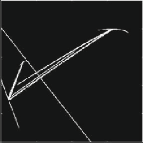
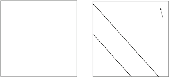
Fig. 4.19
The oligopoly model with intertemporal demand interaction and adaptive adjustment in
the discrete time case. The N-firm symmetric model with iso-elastic price function and linear cost
functions. Parameter values are N
D
8;A
D
1;c
D
0:15;a
D
0:8;ˇ
S
D
0:55. Calculating the
regions that delineate the chaotic attractors. (
a
)HereL
2; the border b
0
and its images T.b
0
/,
T
2
.b
0
/ and T
3
.b
0
/ delineate the region within which the chaotic attractor lies. (
b
)HereL
D
1:2;
now new borders b
1
and b
2
appear. The crossing of the lower part of the chaotic attractor by b
2
leads to new foldings in the boundaries of the chaotic attractor, indicated by the
arrow
D
which L>A=4c. In this case the chaotic attractor crosses the border b
0
between
the regions
2
(see Fig. 4.12), and the images of the portion of b
0
that inter-
sects the attractor, denoted by T
k
.b
0
/, k
D
1;2;3 in the figure, give a delineation of
the chaotic attractor (if the sequence of images is continued by representing T
k
.b
0
/
for increasing values of k, the whole boundary of the attractor will be obtained).
The chaotic attractor shown in Fig. 4.19b is obtained with L
D
1:2,sothat
L<A=4c. In this case, borders b
1
and b
2
also exist, and b
2
crosses the lower por-
tion of the chaotic attractor. This implies that its images determine new foldings
in the boundaries of the chaotic attractor, as can be clearly seen in the upper part
(indicated by the arrow) folded by T.b
2
/. In the cases that we have examined here
the second possible candidate for “folding curves,” namely the locus of vanishing
Jacobians plays no role. This is so since the curve of the vanishing Jacobian does
not intersect the chaotic attractor, and so cannot be used to bound it.
1
and
D
D
4.3.3
Continuous Time Models
In a similar fashion to the discussion of previous models the local asymptotic
stability of the dynamical system (4.31)-(4.32) is examined by linearization. The
Jacobian of the system at the equilibrium has the form

Search WWH ::

Custom Search