Chemistry Reference
In-Depth Information
2
x
0
10
S
0
β
1
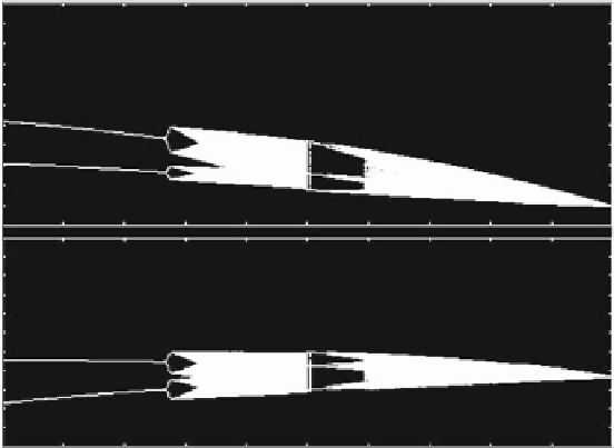
Fig. 4.18
The oligopoly model with intertemporal demand interaction and adaptive adjustment
in the discrete time case. The N-firm symmetric model with iso-elastic price function and linear
cost functions. Bifurcation diagrams with respect to ˇ
S
when the number of firms is increased
to N D 10 and the speed of adjustment is decreased to a D 0:5. Other parameter values are
as in Fig. 4.17. Note that the amplitude of the fluctuating attractors is much reduced compared to
Fig. 4.16 and 4.17
with N
D
4 instead of N
D
3. Now we see that the stable 2-cycles are born at ˇ
S
D
0
and period-doubling followed by period halving occurs at intermediate values of ˇ
S
.
As is commonly observed in adaptive models, the amplitude of the oscillations is
reduced with decreasing values of the speed of adjustment a. This effect is shown
in Fig. 4.18, obtained with the number of firms being increased to N
D
10 and the
speed of adjustment being decreased to a
D
0:5. The other parameters remain as in
Fig. 4.17.
When the asymptotic dynamics is chaotic, it is important to study the size and
the shape of the chaotic attractors inside which the long-run dynamics are ulti-
mately bounded. As already shown in the examples of the previous chapters (see
also Appendix C), the boundaries of the chaotic sets can be obtained by taking the
images of the folding curves, that may be critical curves (loci of vanishing Jacobian)
or the lines of non-differentiability (the borders that separate the different regions
D
.i /
). In our case, the candidates for the “folding curves” are:
The curves of non-differentiability, which are the lines .N
1/x
C
ˇ
S
S
D
A=c
when L>A=.4c/and the lines .N
1/x
C
ˇ
S
S
D
z
1
and .N
1/x
C
ˇ
S
S
D
z
2
when L<A=.4c/;
The curves of vanishing Jacobian, given by
det
J
.1/
.x;S/
D
0.
In Fig. 4.19 two chaotic attractors are shown. Figure 4.19a is obtained with the
parameters N
D
8, A
D
1, c
D
0:15, L
D
2, a
D
0:8, ˇ
S
D
0:55,for
Search WWH ::

Custom Search