Chemistry Reference
In-Depth Information
The results given in this proposition show that for a large set of values of the
cost externality and the adjustment speed a, multiple stable Nash equilibria are
obtained (see the shaded area in Fig. 3.11). Additionally, for sufficiently high values
of the adjustment coefficient a in this area, namely for a>a
p
./, a stable 2-cycle
C
2
coexists with the two stable equilibria E
1
and E
2
. This latter point seems to be
important for the following reason. If the adjustment process converges to the equi-
libria only if initial conditions are chosen from a certain subset of
and otherwise
it cannot be observed, it becomes crucial to obtain information on the relative size
of the set of initial conditions from which players can eventually coordinate their
actions (see Mailath (1998), Fudenberg and Levine (1998)).
We will now turn to the analysis of the global dynamics of the model. Since we
are not able to discriminate among the equilibria E
1
and E
2
on the basis of the
local stability properties, to obtain further information on the stability properties of
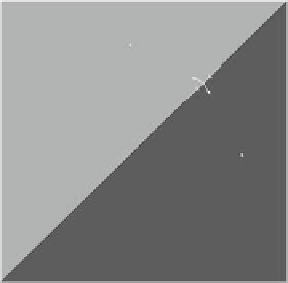
the Nash equilibria we will study their basins of attraction. Figure 3.12 depicts the
basins of the locally stable equilibria E
1
and E
2
for two quite distinct situations.
In Fig. 3.12a, obtained with
D
3:4 and a
D
0:2<1=.1
C
/
D
0:2273, the basins
have a quite simple structure. For initial production quantities in
S
with x
1
.0/ >
x
2
.0/ the adjustment process (3.23) converges to the equilibrium E
1
. On the other
hand, if the reverse inequality holds, then the process converges to the equilibrium
E
2
. Therefore, if firm 1 (firm 2) initially dominates the market in terms of market
share, this property prevails throughout and the equilibrium E
1
(equilibrium E
2
)
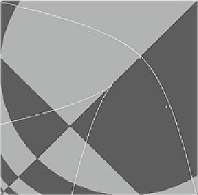
is eventually selected. In contrast to this, the situation shown in Fig. 3.12b, is quite
different. It is obtained with the same value of the cost externality , but with higher
values of the adjustment coefficients, namely a
D
0:5 > 1=.1
C
/
D
0:2273.In
S
1
1
x
2
E
2
x
2
E
2
Δ
Δ
E
S
E
S
Δ
−1
K
Z
0
E
E
1
LC
(
b
)
LC
(
a
)
Δ
−1
Z
2
Z
4
x
1
x
1
0
1
0
1
(a)
(b)
Fig. 3.12
Oligopolies with linear inverse demand function and cost externalities. The case of
duopoly with identical speeds of adjustment. Basins of attraction of the multiple Nash equilibria
(
a
) Simple structure for
0:2. Convergence to either E
1
or E
2
depending on which
firm dominates initially. (
b
) Non-connected basins for
D
3:4 and a
D
0:5, now convergence to
E or E
2
cannot be determined on the basis of which firm dominates initially
D
3:4 and a
D
Search WWH ::

Custom Search