Image Processing Reference
In-Depth Information
V
R
�
-
‚
+
(
)
≈
log
log
R
′ Ψ
+
Ψ
V
RR
�
-
‚
+
(8.16)
≈
log
′
The second term in Equation (8.16) contains spatial frequencies, which are
similar to the spatial frequencies of the incident field One can vary the fre-
quency of the incident plane wave to determine the spatial frequency char-
acteristics of the second term in Equation (8.16) whereas log(
V
/
R
) should stay
the same. The implementation of the cepstral filtering requires that a low pass
filter be applied until the wavelike structure associated with
V
〈Ψ〉 is removed.
The success of the filtering operation depends upon how distinct the spatial
frequencies of
V
〈Ψ〉/
R
′ are from spatial frequencies of log(
V
/
R
). A linear combi-
nation of estimates for
V
acquired in this way will further improve the signal-
to-noise ratio (SNR) of the reconstructed
V
while suppressing any residual
components from the Fourier transform in each of these images.
8.5 two-dIMenSIonAl FIlteRIng MethodS
Once the data from a scattering image has been properly processed as dis-
cussed in the previous section, and mapped into the cepstrum domain, it is
now necessary to filter the data in an attempt to eliminate or at least attenuate
the Ψ “noise” term and obtain a better representation of the original target,
V
(
r
). Since the preprocessed data is now minimum phase as demonstrated in
the previous section, we know, as stated earlier, that one of the main charac-
teristics of minimum phase data is that most of the energy related to
V
(
r
)〈Ψ(
r
)〉
should be located near the origin. This would suggest that some type of low
pass filter should work well if chosen properly. In basic filter theory (Gonzalez
and Woods, 1992; Jackson, 1991), there are two basic types of low pass filters
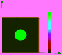
to consider. They are the ideal low pass filter illustrated in Figure 8.3, and
the Gaussian low pass filter illustrated in Figure 8.4. In each of these figures,
a top view, isometric view, and slice or profile view is shown for each filter
u
(a)
(b)
(c)
H
(
u
,
ν
)
1
H
(
u
,
ν
)
0.9
600
1
0.9
0.8
0.7
0.6
0.5
0.4
0.3
0.2
0.1
0
1
0.8
500
400
300
200
100
0
0.7
1
0.5
0.6
0.5
0.4
0
0
0
0.3
100
100
200 200
300 300
400
400
500
500
600
600
0.2
0.1
ν
D
(
u
,
ν
)
0
100 200 300 400 500 600
D
0
0
ν
u
Figure 8.3
Low pass filter. (a) Ideal hard-cut low pass filter 2-D view, (b) low pass filter displayed in 3-D, and
(c) the cross section of ideal low pass filter.


Search WWH ::

Custom Search