Biomedical Engineering Reference
In-Depth Information
b
a
10
50
5
100
0
150
-5
-10
200
-7
187
382
578
773
0
200
400
600
Time (ms)
Time (ms)
c
d
50
100
150
200
−7
187
382
578
773
Time (ms)
f
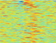
Fig. 7.5
Reordering results on EEG oddball time series. The
solid vertical line
in the raster plots
corresponds to the stimulus onset. The
vertical dashed lines
provide the limits on the time window
used to reorder the data. This time window is manually set around the largest fluctuation of the
evoked response. Embedding was performed with
r
=2
and
σ
=0
.
05
.(
a
) Raster plot of raw time
series; (
b
) Two sample time series; (
c
) 2D embedding of the time series; (
d
) Raster plot reordered
using the first coordinate
f
1
of the embedding
with a high-pass filter at 0.5 Hz (Butterworth zero phase filter, time constant
0.3183 s, 12 dB/oct) and a low-pass filter at 8 Hz (Butterworth zero phase filter,
48 dB/oct). The positive deflection of the P300 wave, in the 3-5 Hz range, is
preserved. Figure
7.5
a presents a raster plot of the data set. The random nature of
the time latency of the P300 is apparent, as first observed in [
15
].
The time series were embedded into a two dimensional space (Fig.
7.5
), after
restricting the time series to a time interval around the largest fluctuation of the
evoked response. This interval was manually defined by visual inspection of the
dataset. It can be noticed that the points are clustered along an elongated 1D
structure, as in the synthetic dataset presented in Fig.
7.4
. The first coordinate can
therefore be used to correctly parameterize the manifold (Fig.
7.5
c) and to order the
time series. By observing the reordered raster plot in Fig.
7.5
d, it appears that the
first coordinate of
f
has correctly captured the latency ordering.
7.3
Model-Driven Approaches: Matching Pursuit and Its
Extensions
The above-presented data-driven approaches require that the data belong to a
low dimensional manifold. However, this is often not the case in practise either


Search WWH ::

Custom Search