Geoscience Reference
In-Depth Information
Ricker wavelet 500 Hz
1
0.5
0
−0.5
0
1
2
3
4
5
6
7
8
9
10
(a)
Time (ms)
Amplitude spectrum of Ricker wavelet 500 Hz
1
0.8
0.6
0.4
0.2
0
0
200
400
600
800
1000
1200
1400
1600
1800
Frequency (Hz)
(b)
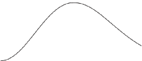
Figure 6.2
Pressure source
f
(
x
,
t
) used for the beamforming experiment. The pressure source is a Ricker wavelet with a 500 Hz
dominant frequency and a time shift of 5 ms.
a)
Pressure time series of the source.
b)
Amplitude spectrum of the source.
minimumwavelength of 2 m. That gives us a seismic res-
olution of 1.55 and 0.51 m, respectively. All numerical
modeling shown in this section is performed using the
finite-element package COMSOL Multiphysics with tri-
angular meshing of nonconstant element size (minimum
element size of 0.0024 m and maximum element size of
1.2 m). This choice was driven by the need to have 5
mesh elements per wavelength. In order to model the
study areas without any seismic reflection at the bound-
aries (i.e., simulate an infinite medium), we use the
convolution perfectly matched layer (C-PML) developed
by Jardani et al. (2010). The thickness of the C-PML is
10 m around the area of interest. The seismic P-waves
are propagated from the source to the fictitious electrodes
located in place of the true seismic sources in the wells
and along the ground surface. For every shot, we record
the macroscopic pressure field,
P
i
(
t
), at each geophone
identified by index
i
located in the wells.
Step 2
: Once the pressure fields have been recorded at
each geophone, we back propagate the pressure fields as
shown in Figure 6.3. Next, we time-reverse the signal
recorded at each geophone ((
P
shifted
(
t
)=
P
recorded
(
T
−
t
),
where
T
is the total recording time or listening time).
Then, we create seismic point sources located at all of
the positions of the virtual geophones and reinject the
reversed seismic signals into the medium. The outgoing
pressure field propagates and interferes constructively
at the original source location (see Figure 6.3). During
this backpropagation, we record the electrical potential
at the electrodes placed in the wells and along the ground
surface. As indicated earlier, the 46 electrodes colocated
with the seismic sources; however, this is not at all a
requirement for this method.
The strength of this technique comes from the fact that
we know exactly at what time and what location the
seismic wave fields focus and interfere constructively. If
the point of focus is located on an interface, we record
an interface response with a greater amplitude than we
would have recorded for a passing wave field crossing
the interface. In fact, the electric potential, caused
by a seismoelectric conversion from a discontinuity in
medium properties, is usually orders of magnitude
smaller than the coseismic field (electrical field giving rise
to an electrical potential only detectable inside the
support of a seismic wave). An example is shown in
Figure 6.2 depicting the dipolar field created by the
beamforming of the seismic waves at point A. This
technique forces the interface response conversion to