Geoscience Reference
In-Depth Information
0
0
10
10
E29
Background
20
20
Background
Anomaly 1
30
A
30
A
40
40
50
50
Anomaly 2
60
60
70
70
80
80
90
B
90
B
E1
E46
100
100
0
10
20
30
40
50
60
0
10
20
30
40
50
60
Offset (m)
(a)
(b)
Offset (m)
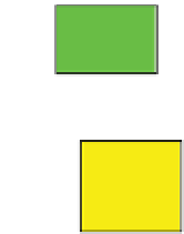
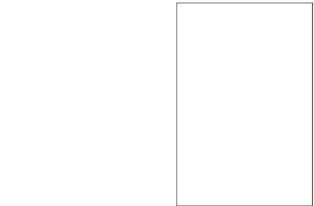
Figure 6.1
Geometry used for the beamforming problem. The medium consists of a homogeneous background model (reference model,
fully saturated) plus two anomalies termed Anomaly 1 and Anomaly 2. These anomalies correspond to areas that are unsaturated
(see Table 6.3). The survey area is surrounded by two vertical wells located on each side. The triangles correspond to the location of the
seismic sources/geophones/electrodes. The spacing between two consecutive sensors is 5 m. The two boreholes have 19 dipoles of
electrodes each, and sets of sensors are located close to the ground surface (5 m deep). The two red-filled circles correspond to the
focusing points used for our numerical experiments. Ei corresponds to the position of electrode i. There are 46 set of sensors in total with
E1 and E46 at the bottom of the two wells.
a)
Reference model (without the two heterogeneities).
b)
Model used for the numerical
simulation with the two heterogeneities. (
See insert for color representation of the figure
.)
Going further, we could scan the subsurface and
“
map
”
in 3D these heterogeneities.
We solve the partial differential equations for the
mechanical and electrical problems in the frequency
domain as explained in Chapter 4.
Table 6.1
Petrophysical properties for the background
and Anomalies 1 and 2.
Property
Background Anomaly 1 Anomaly 2
22 × 10
9
22 × 10
9
22 × 10
9
Undrained bulk
modulus
K
u
(Pa)
V
p
(m s
−
1
)
P-wave velocity
3093
3093
3093
6.1.2 Beamforming technique
The beamforming technique enables us to focus seismic
energy at a desired location and at a known time. As dis-
cussed in Sava and Revil (2012), the velocity model does
not need to be perfectly known. In the present case, how-
ever, we will assume that it is perfectly known. Seismic
beamforming is based on time reversal process and is
accomplished in two steps:
Step 1
: On a finite-element grid, we choose the point
of focus and we construct a fictitious seismic point source
at that location. In this case, the seismic source is a
Ricker wavelet with a dominant frequency of 500 Hz
(Figure 6.2). It contains energy up to about 1500 Hz.
Using a constant seismic P-wave velocity of 3100 m s
−
1
,
we obtain a dominant wavelength of 6.2 m and a
Excess charge density
Q
V
0.20
2.0
6.7
(C m
−
3
)
m
2
)
Log (permeability,
k
−
12
−
14
−
16
Skempton coefficient
B
0.65
0.65
0.65
Average density
ρ
(kg m
−
3
)
2300
2300
2300
10
−
3
10
−
3
10
−
3
Hydraulic viscosity of pore
fluid
η
f
(Pas)
(S m
−
1
)
Conductivity
σ
1
0.01
0.001
Saturation
s
w
(
—
)
1
0.10
0.03
If we scan various points in the medium, this technique
would enable us to identify whether the point of focus
is located in the vicinity of such heterogeneity or not.