Environmental Engineering Reference
In-Depth Information
2
φ
t
1.5
1
0.5
1000 1500 2000 2500 3000
t
500
0.5
1
1.5
2
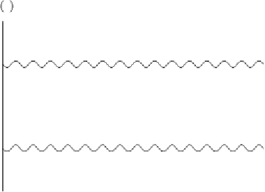
Figure 3.21. Examples of time trajectories corresponding to periodic potential
V
1
(
φ,
t
)inEq.(
3.62
) with
α
=
0
.
15 and
ω
p
=
π/
100. Notice that no transitions
occur.
deterministic dynamics expressed
d
d
t
=
φ
2
)
(1
−
φ
−
α
sin(
ω
p
t
)
.
(3.63)
It is observed that in the absence of noise the state of the system remains confined
in either one of the two potential wells, depending on the initial condition. The only
effect of the deterministic forcing is to induce periodic fluctuations around the steady
states,
1.
As the periodic term in (
3.62
) is linear in
φ
m
,
1
=
1or
φ
m
,
2
=−
V
but not
the curvature of the potential, which is proportional to the second-order derivative.
Therefore, in the presence of both the random and the deterministic forcings, i.e.,
when the dynamics are regulated by
d
φ
, it is able to alter the height
d
t
=
φ
2
)
(1
−
φ
−
α
sin(
ω
p
t
)
+
ξ
gn
(
t
)
,
(3.64)
the mean transition rate is
2
φ
b
2
φ
m
d
2
V
d
d
2
V
d
−
φ
φ
1
s
gn
[
e
−
V
+
α
sin(
ω
p
t
)]
−
1
(
t
)
t
c
W
(
t
)
=
.
(3.65)
2
π
We recall that Eq. (
3.65
) assumes that
t
c
t
iw
(in our example
ω
p
=
π/
100
<
t
iw
=
2).
Equation (
3.65
) shows how the periodic forcing alternately increases or decreases
the probability of transition from a well to the other (see Fig.
3.22
). This periodic
alternation is a key aspect of stochastic resonance. In fact, when the semiperiod
1
/
π/ω
p
of the periodic modulation of the potential [Eq. (
3.62
)] is comparable to the mean
transition time
of the stochastic process, it is likely that periodic and random
forcing cooperate to induce transitions. In other words, the transition probability is
t
c


Search WWH ::

Custom Search