Noise-induced phenomena in zero-dimensional systems - Noise-induced Phenomena in the Environmental Sciences - page 82

V 1

0.4

0.2

2 φ 2 1 1

0.2

V 1 V 1

0.4 0.4

0.2 0.2

2 φ 2 φ

2 1 1 2 1 1

0.2 0.2

V 1

0.4

0.2

φ

2 1 1 2

0.2

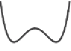
Figure 3.20. Time behavior of the periodic potential V 1 ( φ, t )inEq.( 3.62 ), with

α = 0 . 15 and ω p = π/ 100. The panels refer to t = 0, 50, 100, and 150 time units,

respectively.

Equation ( 3.61 ) shows how the mean transition rate depends on the noise strength,
the height of the potential barrier, and the curvature of the potential at the points of
maximum and minimum. Moreover, the crossing times are exponentially distributed
with mean ( Gardiner , 1983 ). This property is used in the detection methods

presented in the following sections.
If we now add the last ingredient, namely the periodic forcing, the deterministic
potential becomes

t c

V 1 ( φ, t ) = V ( φ ) + αφ sin( ω p t ) , (3.62)

where ω p are the amplitude and frequency of the periodic forcing. In models

of stochastic resonance this forcing is typically “weak” in the sense that it is not able
to induce transitions between the two wells (i.e.,

α and

V ). Therefore the effect of
the periodic forcing is to periodically alter the shape of the potential, with the effect
of alternately reducing or increasing the height of the potential barrier with respect
to each well. Figure 3.20 shows the effect of the periodic forcing on the potential
function for the example presented in this section (with

α<

α = 0 . 15 < V = 1 / 4and

ω = π/ 100), and Fig. 3.21 shows an example of the time series generated by the p