Noise-induced patterns in environmental systems - Noise-induced Phenomena in the Environmental Sciences - page 266

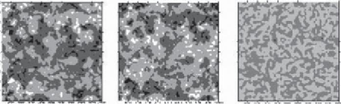
Figure 6.12. Emergence of stationary patterns of prey [ A 1 (left), A 2 (center)], and
predator ( A 3 , right) biomass in the case with μ = β =

=− 0 . 01, μ = 2, 1, ν = 1,

10 − 3 , 10 − 16 , D 0 . 01, ν 0 = ( ω 0 / 2 π ) = α = 0 . 1, s 1 = s 2 = s 3 = 0 . 5 × = 0 . 01, γ =

10 2 . Darker gray corresponds to higher biomass densities.
Figure taken from Spagnolo et al. ( 2004 ).

10 − 2 , γ =

3 × 2 . 05 ×

that is correlated with both preys (Fig. 6.12 ). Conversely, if the initial distribution of
the two preys has a peak and the predator has a homogeneous initial condition, the
system converges to a configuration with strong cross correlation between the two
preys (i.e., coexistence of A 1 and A 2 ). These patterns emerge when the noise intensity
exceeds a certain critical level. However, patterns disappear for relatively large values
of the noise intensity, consistent with the theory of stochastic resonance (Chapters 3
and 5).

6.8 Spatiotemporal coherence resonance in excitable plankton systems
In this section we consider a spatially extended version of the excitable phytoplan
kton-zooplankton systempresented in Chapter 4 (Subsection 4.8.4 ). We recall that it is
a systemwith three state variables: phytoplankton susceptible to infection Z s , infected
phytoplankton Z i , and zooplankton Z z . Phytoplankton biomass Z s , i undergoes logistic
growth and is harvested by the zooplankton. Moreover, Z s is turned into Z i (infection
process), while Z i undergoes disease-induced mortality. The zooplanton biomass
grows proportionally to the rate of phytoplankton harvesting and decays proportionally
to Z z . Sieber et al. ( 2007 ) investigated the effect of multiplicative noise on the temporal
dynamics of this system and found that coherence resonance may emerge from the
cooperation between noise and the underlying nonlinear deterministic dynamics close
to a Hopf bifurcation. Thus noise is able to unveil a characteristic time scale of the
deterministic dynamics and induce coherent periodical fluctuations in the time domain.
We now consider a 2D extension ( Sieber et al. , 2007 ) of this system with spatial
coupling expressed by a diffusion term:

∂ Z k ( r , t )

2 Z k ( r

= f k [ Z s ( r , t ) , Z i ( r , t ) , Z z ( r , t )] + D ∇ , t ) + Z k ( r , t ) ξ k ( r , t ) , (6.29)

∂

t