Noise-induced patterns in environmental systems - Noise-induced Phenomena in the Environmental Sciences - page 267

t = 25 t = 26 t = 26.5 t = 31

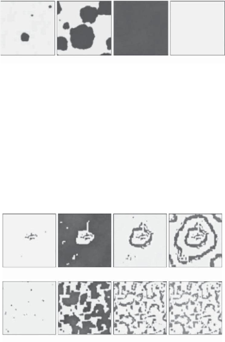
Figure 6.13. Spatiotemporal evolution of the excitation of susceptible biomass
Z s ( r 10 − 4 , and the same parameters

as in Subsection 4.8.4 in Chapter 4. Darker gray corresponds to higher biomass
densities. Figure taken from Sieber et al. ( 2007 ).

10 − 2 , s gn = , t ) calculated with D = 5 × 2 ×

with k t )] are defined as the right-

hand sides of Eqs. ( 4.80 ) in Chapter 4; D is a diffusion coefficient, and

= s , i , z . The functions f k [ Z s ( r , t ) , Z i ( r , t ) , Z z ( r ,

ξ

k is a
zero-mean Gaussian noise with intensity s gn and no autocorrelation either in space or
time. Numerical simulations of ( 6.29 )( Sieber et al. , 2007 ) show that with adequate
levels of noise the temporal dynamics of the spatial mean exhibit periodic fluctuations
similar to those detected in the zero-dimensional model (Subsection 4.8.4 , Chapter 4).
The random forcing displaces the system from its homogeneous rest state by inducing
local excitations, which then spread over the whole domain as an effect of diffusion.
Thus, depending on the diffusion coefficient and the size of the domain, a state of
global excitation may be reached before the system returns back to its homogeneous
rest state, as shown in Fig. 6.13 . Therefore both diffusion and local excitations induced

t = 55 t = 62 t = 85 t = 200

t = 25 t = 37 t = 67 t = 200

10 − 4 (top row) Figure 6.14. Emergence of stationary patterns of Z s with s gn = 3 ×

10 − 4 (bottom row) and the same parameters as in Fig. 6.13 .Darker
gray corresponds to higher biomass densities. Figure taken from Sieber et al. ( 2007 ).

and s gn = 5 ×