Information Technology Reference
In-Depth Information
An interesting case is also that of a highly randomized lattice; Fig. 3 shows that, in
the case f=1.6, the number of different attractors which are reached from 1000
random initial conditions starts to grow at a much higher r value (beyond 0.4) than in
the regular case, and that the peak reached around r=0.5 corresponds to a number of
attractors which is much smaller than in the regular case. In the case r=0.5 there are
two major attractors, with equal basins of attraction, which together cover about 80%
of the initial conditions.
As far as transients are concerned, there is a nearly linear increase as r grows; this
is similar to what is observed also in the regular case, but the maximum transient
duration is much higher (transient duration also displays a very high variance in the
region near 0.5).
bm1300
bm1300
1200
300
1000
250
Dimensions
first attractor
800
200
600
Dimensions
second
attractor
Other
attractors
150
400
100
50
200
0
0
0
0.2
0.4
0.6
0.8
1
0.4
0.45
0.5
0.55
0.6
r
r
Fig. 3.
Majority rule on a randomized graph (f=1.6): average number of attractors reached
starting from 1000 random initial conditions (left); fraction of initial conditions which are
attracted by the largest, second largest and "all the other" stable points (right). All the variables
are shown as a function of r (n=1000; k=10)
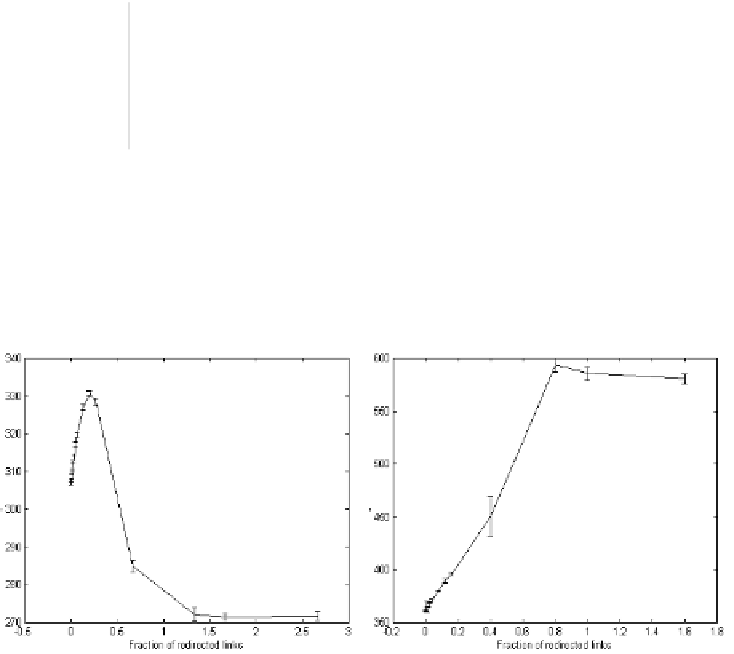
Fig. 4.
Duration of transients (time stpes needed to reach the fixed point) as a function of the
degree of randomness at k=6 (left) and k=10 (right). Each point is the average of the values
obtained from 10 different networks; n=1000, 1000 different initial conditions for each net
Finally, it is also interesting to observe the behaviour of the transients as a function
of the degree of randomness. At high k values their duration increases with increasing