Environmental Engineering Reference
In-Depth Information
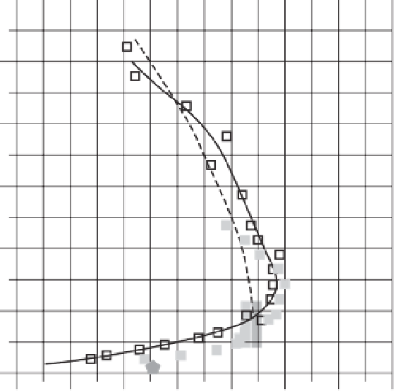
Hinze (1975)
core region
of a pipe-flow
1.2
x = 1500mm (H = 75mm)
z
/
δ
x = 1500mm (H = 8mm)
Fit (x = 1500mm, H = 8mm)
1.0
0.8
Ludwieg and Johnson
(Rotta, 1964)
0.6
0.4
Schlichting (1997)
Launder (1978)
0.2
Raupach et al. (1996)
0.0
0.0
0.2
0.4
0.6
0.8
1.0
1.2
1.4
Sc
t
=
ν
t
/
K
z
Figure 6.8
Turbulent Schmidt number as a function of height in the ABL, normalized by the boundary layer thickness (Modified
with permission from Koeltzsch, K. (2000) The height dependence of the turbulent schmidt number within the boundary layer.
Atmospheric Environment
, 34, 1147-51.).
users understand the difficulties and pitfalls in CFD. This
requires experience in CFD but also an understanding
of the particular applications area. A crucial point is to
ensure that before starting any simulation the questions to
be answered from the simulation are clearly stated. Once
this is done the data that is necessary to answer these
questions can be outlined and only once this is available
should the modelling start. The modelling complexity
should be established based on the data available. A
complex model that has insufficient data for validation
cannot be relied upon to give well-founded conclusions.
Key areas for future research that will open up greater
application for CFD in environmental flows are: large
eddy simulations for a more realistic representation of
turbulence; improved roughness models and increased
computing power. The latter will allow for much larger
meshes and multiple runs to be used, which opens up the
possibility of automatic calibration, numerical optimiza-
tion and parametric uncertainty analysis.
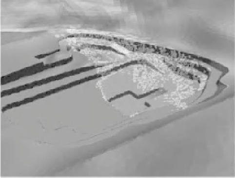
Figure 6.9
Contours of dust deposition within an open-cast
mine (Modified with permission from Silvester, S.A., Lowndes,
I.S. and Hargreaves, D.M. (2009) A computational study of
particulate emissions from an open pit quarry under neutral
atmospheric conditions.
Atmospheric Environment
, 43,
6415-24.).


Search WWH ::

Custom Search