Environmental Engineering Reference
In-Depth Information
invariably, be shorter than the equivalent from the wind
tunnel. Sampling periods of 10 minutes or 1 hour are
not uncommon in wind-tunnel experiments in order
to capture the extremes of the wind speed record. To
generate an equivalent set of data from a CFD simulation
is unrealistic - maybe a minute could be simulated by
LES at the levels of spatial and temporal detail required.
This limitation highlights a major issue for the use of CFD
to predict wind loads on structures as it is not currently
possible to extract meaningful statistics from such short
datasets. With an eye on the future increases in computer
power, Xie and Castro (2008) have developed time and
space-varying inlet conditions, which can simulate the
statistical nature of a real wind in order to allow the
gustiness to be included in LES simulations.
There is, however, some encouragement for CWE prac-
titioners. With improvements in technology that allow
fluid-structure coupling, there is evidence (Owen
et al
.,
2006) that when the motion of the structure contributes
the dominant frequency to the flow, then even unsteady
RANS (but, ideally, LES) models can produce meaning-
ful results. This observation is especially true for tall,
flexible structures where inaccuracies in flow separa-
tion on the roof play but a small part in the structural
response (Braun and Awruch, 2009). Further, CFD for
pedestrian-level wind-environment simulations is rou-
tinely used by the building-services industry because the
predictions of velocity around buildings are suitable for
comparative studies (for example, with and without a
new, iconic building).
The other main area in which CFD is used in environ-
mental modelling is in studies of air-pollution dispersion.
Here again there are issues as suggested by Cowan
et al
.
(1997). The trials reported by themwere of calculations of
pollutant concentrations for a variety of well-documented
cases, most of which have experimental verification. They
were carried out independently by a number of different
organizations, using the same computer code. The differ-
ences between the calculations were thus in the realms of
grid generation, numerical schemes etc. The results pro-
duced by different investigators were found to vary very
significantly (often by an order of magnitude or more).
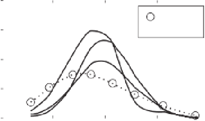
Typical comparisons are given in Figure 6.7.
In other work, Riddle
et al
. (2004) conduct a compar-
ison between a commercial CFD code and a standard
Gaussian plume model, ADMS. They found significant
differences between the two. Indications from their work
and that of Tominaga and Stathopoulos (2007) were that
the CFDmodel had to be tuned to agree with the Gaussian
plume model by means of the turbulent Schmidt number,
2
Expt
CFD
1.5
1
0.5
0
−
3
−
2
−
1
y/H
0
1
Figure 6.7
Concentration profiles obtained from CFD
implementations by different investigators compared with the
experimental data for one of the test cases in Cowan
et al
.
(1997) (Reproduced with permission from Cowan, I.R.,
Castro, I.P. and Robins, A.G. (1997) Numerical considerations
for simulations of flow and dispersion around buildings.
Journal of Wind Engineering and Industrial Aerodynamics
,
67-68: 535-45).
which effectively relates the local turbulence level to the
rate of pollution dispersion, on a case-by-case basis.
This situation is further complicated by the fact that the
turbulent Schmidt number in reality varies with height
in the unobstructed ABL - see Figure 6.8 (taken from
Koeltzsch, 2000). However, there are instances where
the use of CFD has a distinct advantage over the Gaus-
sian plume approach. Silvester
et al
. (2009) demonstrated
that the retention of dust in open-cast mines was far
more accurately modelled using CFD, due to the complex
topology involved (Figure 6.9).
These results serve as a warning against placing too
great a reliance on the accuracy of any one calculation
that does not have some sort of experimental validation.
The unverified use of CFD codes to reduce the costs of
physical model tests can, if great care is not used, simply
be to produce results that are unreliable. These points are
further discussed and emphasized by Castro and Graham
(1999). It must be concluded that that CFD and physical
modelling should be seen as complementary technologies
that should be used in conjunction with one another to
varying degrees for any particular situation.
6.4 Conclusions
Computational fluid dynamics has many applications in
environmental flows as outlined here but there are still
challenges to be faced to increase its accuracy and ability
to deal with more complex situations. It is also vital that


Search WWH ::

Custom Search