Environmental Engineering Reference
In-Depth Information
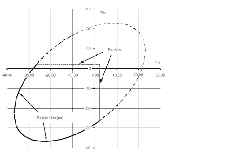
Fig. 3.14 Drucker-Prager or Rankine failure in biaxial stress
Tension meridian:
þ
b
2
2
r
2
ðÞ¼
b
0
þ
b
1
j=
f
c
;
1
j=
f
c
;
1
Convexity condition:
r
1
=
2
<
r
2
r
u
INT
ð
Þ
r
1
(elliptical interpolation for - 60
u
INT
þ
60
)
The principal meridians meet at the apex of the cone and therefore produce two
additional free parameters - the “high” tension meridian stress f
Z
and the “high”
compression meridian stress f
D
- in order to determine the coefficients a
0
,a
1
,a
2
and b
0
,
b
1
,b
2
[41]. See [8] for more details.
Whereas the strength values f
c,1
,f
c,2
and f
ct
have to be obtained from tests, the “high”
meridian stresses should lie in the region of the largest hydrostatic compression action
effect of the structure being investigated. The idea is that the five-parameter model
approximates the Von Mises model for these limit states.
3.6.3 Three-phase model
The aim of this model is to formulate a continuously differentiable approach -
and hence an approach suitable for numerical analyses - which can be adapted
to the test results available with the help of a few physically sensible parameters