Information Technology Reference
In-Depth Information
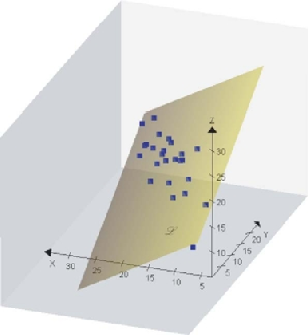
Figure 3.6
Interpolated sample points represented in terms of the three Cartesian axes.
> points(x = -6.0009, y = 0.2896, pch = 1, col = "blue",
cex = 2, lwd = 2)
> draw.arrow(col = "black", length = 0.15, angle = 15, lwd = 1.75)
> arrows(-6.0009, 0.2896, -6.0009*3, 0.2896*3, col = "black",
length = 0.15, angle = 15, lwd = 1.75, lty = 2)
> points(-6.0009*3, 0.2896*3, pch = 16, col = "red", cex = 0.8)
> draw.text(string = "outlier?", cex = 0.6)
The function
vectorsum.interp
is available for performing most of the above actions
in a single function call.
In the next section we show in detail how to equip the PCA biplot with axes that can
be used for prediction - that is, to allow reading off of variable values associated with
the respective samples.
3.2.3 Prediction biplot axes
To illustrate the construction of a prediction biplot axis, the first Cartesian axis (
X
)of
the Table 3.3 data will be used.