Information Technology Reference
In-Depth Information
d
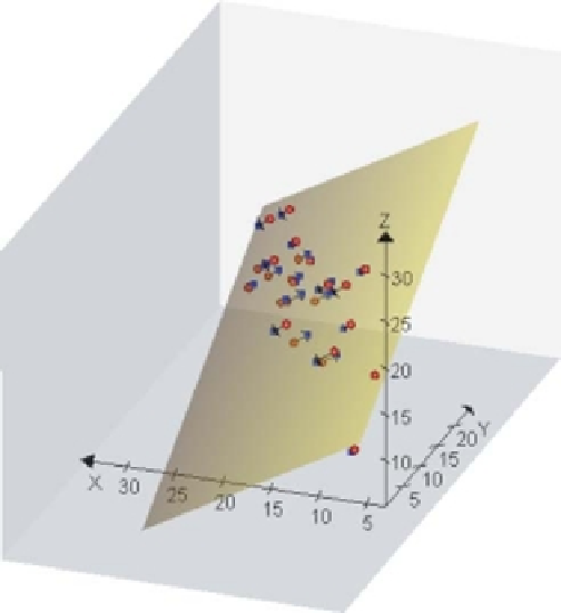
2D Biplot plane through
full 3D space
Figure 3.5
Projection of three-dimensional sample points onto the two-dimensional
biplot space
L
. Red points in full space are projected orthogonally onto the blue points
in
L
such that the sum of the squared distances
(indicated by the black arrows) is
minimized. Actual distances in the full space are denoted by
d
; approximated distances
in
L
denoted by
ε
δ
. The plane of best fit passes through the centroid of the data.
that the calibrations of the axes are in terms of the original units used in Table 3.3.
However, several features of Figure 3.10, for example the number of calibrations on each
biplot axis, need to be fine-tuned. We will attend to fine-tuning of biplots in subsequent
sections.
Recall from Section 2.6 that the biplot axes in Figure 3.10 cannot be used for reading
off the
X
,
Y
or
Z
value of any given sample point. However, as we have seen in Section
2.6, the interpolation calibrations can be used to determine the position of any new point
in the biplot space using the vector-sum method. We illustrate this method step by step
in Figure 3.11, introducing some functions for interactively enhancing biplots.
Figure 3.11 is the result of the following code:
> draw.arrow(col = "red", length = 0.15, angle = 15, lwd = 1.75)
The function
draw.arrow
is called three times, using the mouse to select the beginning
and the end of the arrow.
> draw.polygon(vertex.points = 3, border = "blue", lwd = 1.75)
The function
draw.polygon
draws the polygon as selected by the mouse and returns
the coordinates of the polygon's centroid as (
−
6.0009, 0.2896).