Information Technology Reference
In-Depth Information
0.1
−
0.01
0.15
−
0.02
−
0.04
−
0.1
0.1
−
0.02
RAC
0.05
Gaut
−
0.005
AtMr
−
0.02
−
0.05
−
0.005
0.01
CrJk
0.05
CmRb
−
0.01
0.02
KZN
InAs
DrgR
AtMr
CmRb
0.02
0.2
InAs
DrgR
−
0.02
CmAs
0.01
WCpe
0
0.1
PubV
Mrd
CmAs
Arsn
BRs
−
0.1
−
0.01
BNRs
Rape
−
0.02
Mpml
NWst
FrSt
Limp
−
0.01
0.005
−
0.05
NCpe
0.01
0.05
0.005
ECpe
0.02
−
0.05
Arsn
AGBH
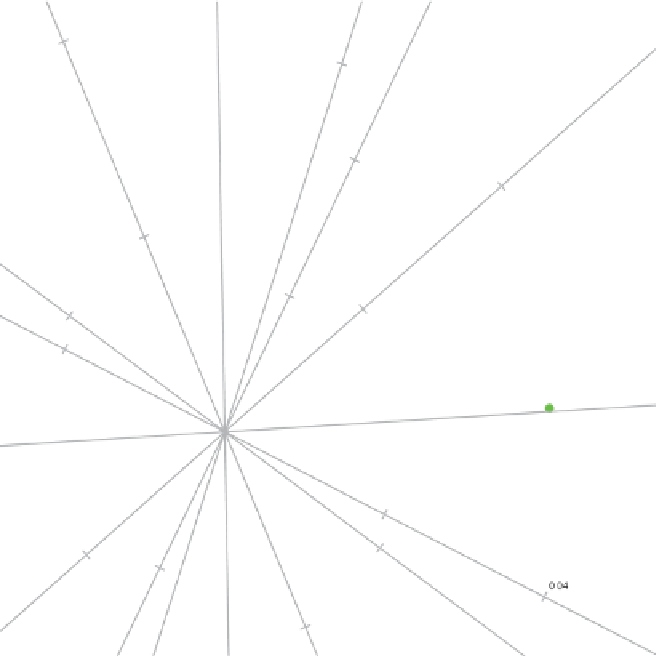
Figure 7.4
Two-dimensional CA biplot for the 2007/08 crime contingency table,
constructed from the first two columns of
U
1
/
2
1
/
2
. Columns are represented
and
V
by axes. Calibrations on axes are in terms of
R
−
1
/
2
(
X
−
E
)
C
−
1
/
2
, that is, proportional
to Pearson residuals.
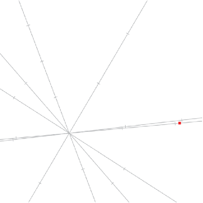
directly in terms of Pearson residuals by incorporating the factor
n
1
/
2
directly in the
calibrations. Setting in
cabipl
the argument
PearsonRes.scaled.markers = TRUE
provides axes calibrated in terms of Pearson residuals. The resulting biplot is shown in
Figure 7.6, and its associated overall quality is a satisfactory 87.84% (see Table 7.11).
The sample predictivities and axis predictivities in Tables 7.12 and 7.13 are generally
referred to as the row qualities and column qualities, respectively (see Greenacre 2007).
The two-dimensional axis predictivities of
AtMr
,
BNRs
,
BRs
,
CmAs
and
Mrd
show that
these axes should be used with caution in a two-dimensional biplot. Increasing the biplot
dimension to 3 leads to a considerable increase in the axis predictivities of
AtMr
,
CmAs
and
Mrd
. In two dimensions the sample predictivities are high apart from moderate
values for
FrSt
and
KZN
.