Information Technology Reference
In-Depth Information
0.1
1
0.15
4
-0.02
0.1
2
RAC
0.05
Gaut
AtMr
-0.005
-0.02
-0.05
-0.005
0.01
CrJk
0.05
CmRb
-0.01
0.02
KZN
InAs
DrgR
CmRb
0.02
WCp
DrgR
0.2
AtMr
-0.02
InAs
0.01
0
0.1
PubV
Mrd
CmAs
CmAs
Arsn
0
BRs
BNRs
-0.1
-0.01
Rape
-0.02
Mpml
NWst
FrSt
-0.01
0.005
-0.05
NCpe
Limp
0.01
0.05
0.005
-0.04
ECpe
0.02
-0.05
Arsn
AGBH
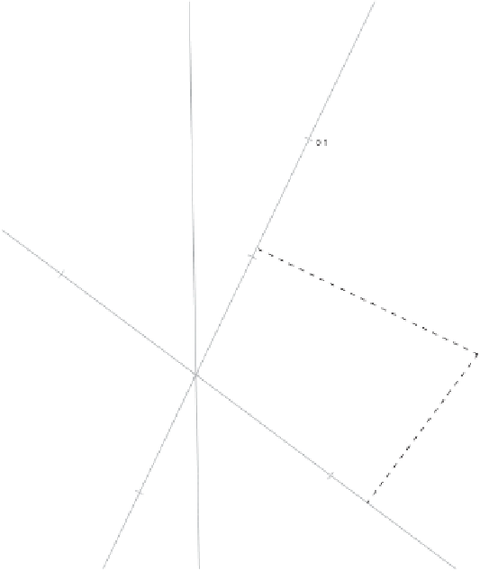
Figure 7.5
Two-dimensional CA biplot for the 2007/08 crime contingency table,
constructed from the first two columns of
U
1
/
2
1
/
2
. Columns are represented
and
V
by axes. Calibrations on axes are in terms of
R
−
1
/
2
(
X
−
E
)
C
−
1
/
2
, that is, proportional
by a factor of
n
1
/
2
to Pearson residuals. It is shown how to obtain these predictions for
the Western Cape province.
We now illustrate the CA biplot resulting from the SVD
R
−
1
/
2
(
X
−
E
)
C
−
1
/
2
=
U
V
but plotting
U
2
. The biplot in Figure 7.7
is obtained by specifying the arguments
ca.variant = "PearsonResB"
and
Pear-
sonRes.scaled.markers = FALSE
in our function
cabipl
.
Although the predictions made from Figure 7.7 are exactly those obtained from
Figure 7.5, the biplot in Figure 7.7 differs in a very obvious way from that in Figure 7.5:
the row points are squeezed towards each other, making graphical prediction difficult.
There is an easy way to address this problem: setting argument
lambda = TRUE
utilizes
the lambda tool described in Section 2.3 by requiring lambda to satisfy
1
/
2
1
/
and
V
instead of
U
and
V
p
tr
(
VV
)
q
tr
(
U
λ
=
2
U
)
.
(7.52)