Information Technology Reference
In-Depth Information
Ves
D
V
esD
180
180
300
300
160
160
1
40
140
350
350
1000
1000
120
120
1200
1200
1400
1400
1600
1600
400
1800
400
1800
FibL
FibL
100
100
450
45
0
80
80
Obul; n
=
20
Oken; n
7. (C hull)
Opor; n
=
10
=
VesL
VesL
0
0.2
0.4
0.6
0.8
1
1.2
1.4
1.6
1.8
0
1
2
3
4
5
6
7
8
9
10
VesD
VesD
180
180
300
300
160
16
0
140
1
40
350
350
1
000
1000
12
0
120
1
20
0
1200
14
0
0
14
00
1600
1600
400
1
8
0
0
400
1800
FibL
FibL
100
100
450
450
80
80
VesL
VesL
0
0.5
1
1.5
2
2.5
3
3.5
4
0
0.5
1
1.5
2
2.5
3
3.5
4
4.5
5
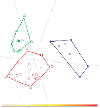
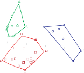
Figure 4.12
CVA biplots with density surfaces and 0.99-bags for each group: (top left)
all samples used for the density surface; (top right) density surface for
Opor
; (bottom
left) density surface for
Oken
; (bottom right) density surface for
Obul
.
In Figure 4.12 we enhance the biplot with various density surfaces by consecutive calls
to
CVAbipl.density
. In these calls we assign the argument
specify.density.class
the values
"allsamples"
,
"Opor"
,
"Obul"
and
"Oken"
to obtain the four biplots
shown in Figure 4.12.
A biplot should always be considered together with the various measures of fit. When
considering the measures of fit for the three variable
Ocotea
CVA biplots, we must keep
in mind that, since we have three groups, the canonical means are exactly represented in
a two-dimensional space. In Tables 4.4 - 4.11 we give the output of the following call to
obtain detailed information to complement interpretation of the CVA biplots:
CVA.predictivities(X = Ocotea.data[,3:5],
X.new.sample = c(134,375,1170), G = indmat(Ocotea.data[,2]),
weightedCVA
= "weighted")