Information Technology Reference
In-Depth Information
CVAbipl(Ocotea.data[,3:5], X.new.samples = matrix(c(134,375,1170),
nrow = 1), G = indmat(Ocotea.data[,2]), weightedCVA =
"weighted", means.plot = TRUE, colours = c("red","blue",
"green"), pch.samples = 0:2, pch.samples.size = 1.25,
label = FALSE, pos = "Hor", line.type = rep(1,3),
line.width = rep(2,3), offset = c(-0.2, 0.05, 0.1, 0.2),
n.int = c(5,10,5), pch.means = c(15,16,17),
pch.means.size = 1.5, side.label = rep("right",3),
pos.m = c(4,4,4), offset.m = c(-0.1, -0.1, 0.1),
parplotmar = c(3,3,3,3), alpha = 0.99, conf.alpha = 0.99,
conf.type = "with.n.factor", specify.bags = 1:3,
legend.type = c(TRUE,TRUE,TRUE), pch.new.col = "black",
pch.new = 8)
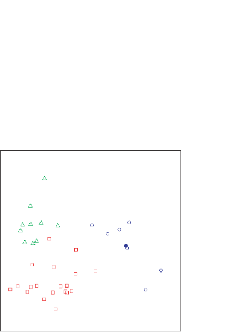
Figure 4.11 clearly shows that the three confidence circles are well separated and that
the specimen of unknown origin lies almost on the perimeter of the confidence circle
around the mean of
Opor
.
VesD
180
300
160
Unknown specimen
140
350
120
1000
1200
1400
1600
1800
400
FibL
100
80
Obul; n
=
20
Oken; n
=
7. (C hull)
Opor; n
450
=
10
VesL
Figure 4.11
CVA biplot for the three-variable
Ocotea
data with 99% confidence cir-
cles drawn about each group mean. For comparison purposes 0.99-bags are also shown
(convex hull for the
Oken
group).