Environmental Engineering Reference
In-Depth Information
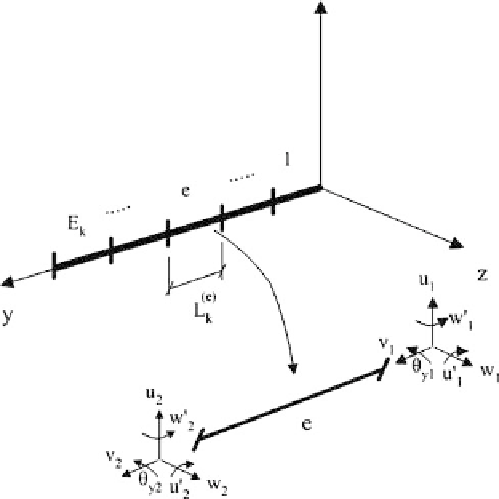
Figure 3 : The fi nite element description of a beam.
Because the equations are in integral form, all calculations can be fi rst carried
out at element level and then proceed with the assembly. For example, the mass
matrix will take the form:
⎛
⎞
⎛
⎞
∫
∫
T
∫
∫
T
M
=
d
y
d
A
r
N
II SN
−
d
y
d
A
r
N
′
II S N
⎜
⎟
⎜
⎟
e
e
s
e
e
s
e
⎝
⎠
⎝
⎠
L
A
L
A
e
e
The fi nal result, after assembling the element matrices will have the usual form:
Mu
ˆ
+=
Ku
ˆ
Q
(9 )
The above system is integrated in time by a marching scheme. In most cases
Newmark's second order scheme is suffi cient. For stiff problems higher order
schemes of the Runge-Kutta type can be also applied [15].
4 Multi-component systems
Next we consider a combination of several beams possibly in relative motion. By
taking each component separately, we need fi rst to include its motion and then add
appropriate compatibility conditions that ensure specifi c connection constraints.
This kind of splitting and reconnecting constitutes the so-called multi-body
approach [ 16- 18 ].
4.1 Reformulation of the dynamic equations
Motions are introduced by assuming that each component undergoes rigid motions
defi ned by the position of its local system [O;
xyz
] with respect to a global (inertial)
Search WWH ::

Custom Search