Environmental Engineering Reference
In-Depth Information
1.6.2 CDF transform approach
Let (Y
1
, Y
2
, …, Y
d
) denote multivariate non-normally distributed random variables. One
well-known CDF transform approach for constructing a valid multivariate distribution for
these random variables is
1. Define
=
()
X
Φ
1
F Y
(1.100)
i
i
i
where Φ
−1
(⋅) = inverse standard normal CDF and Fi(⋅)
i
(⋅) = CDF of Yi.
i
. By definition, (X
1
,
X
2
, …, X
d
) are
individually
standard normal random variables. That is, the histogram
of any component, Xi,
i
, will look normal (bell-shaped).
2. Assume (X
1
, X
2
, …, X
d
) follows a multivariate standard normal distribution as defined
necessarily follow a multivariate standard normal distribution even if each component
is standard normal. For example, if the scatter plot of Xi
i
versus X
j
shows a distinct
nonlinear trend, then the multivariate normal distribution assumption is incorrect.
You can apply the Mahalanobis distance test in Section 1.4.3 as well. The entries in the
correlation matrix
C
in
Equation 1.56
are the Pearson moment-product correlations
among (X
1
, X
2
, …, X
d
). Recall that for multivariate standard normal (X
1
, X
2
, …, X
d
),
the Pearson and Spearman (rank) correlations are nearly identical. Together with the
fact that the rank correlation between (Xi,
i
, X
j
) is identical to that between (Yi,
i
, Y
j
), the
entries in
C
are nearly the same as the rank correlations among (Y
1
, Y
2
, …, Y
d
).
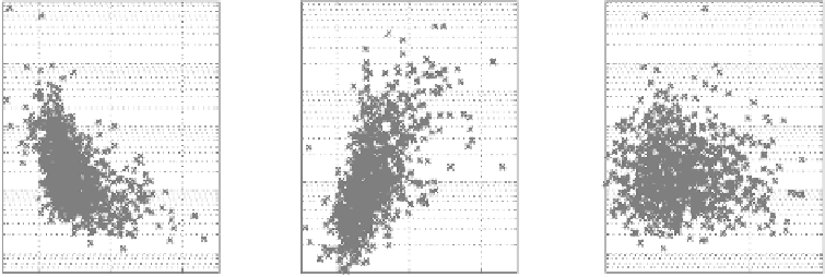
1.6.3 estimation of the marginal distribution of Y
These 1000 data points have full multivariate information: each data point has known (Y
1
,
Y
2
, Y
3
) values. In contrast, incomplete multivariate information will contain data points
such as (Y
1
, Y
2
, ?), (Y
1
, ?, Y
3
), and (?, Y
2
, Y
3
). The question marks denote unknown values.
The treatment of incomplete multivariate information is presented in Section 1.7. The mul-
tivariate data points are simulated using the procedure discussed in Section 1.6.5, with the
10
3
10
3
10
3
10
2
10
2
10
2
10
1
10
1
10
1
10
0
10
0
10
-1
10
-1
10
0
0
2
Y
1
= LI
4
0
2
Y
1
= LI
4
10
0
10
2
exp(Y
3
) =
S
t
Figure 1.25
Simulated multivariate datasets for non-normal (Y
1
, Y
2
, Y
3
).
Search WWH ::

Custom Search