Evaluating reliability in geotechnical engineering - Risk and Reliability in Geotechnical Engineering - page 135

0.250

0.200

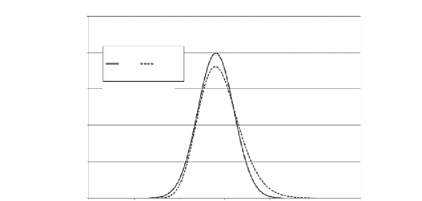
Normals Lognormal

0.150 Average s u = 14 kPa

Standard deviation = 2 kPa

0.100

0.050

0.000

0 5 10 15

s u (kPa)

20 25 30

Figure 3.3 Normal and lognormal distributions, or PDFs.

x is the value of the variable
σ is the standard deviation
x is the average value of x

Equation 3.4 gives the probability for a single value of x . The normal distribution curve
shown in Figure 3.3 was developed by calculating probabilities of values of s u ranging from
0 to 30 kPa, plotting these values against the value of s u , and drawing a smooth curve
through the values.
The Excel function NORMDIST was used to calculate the normal distribution curve
shown in Figure 3.3 . This Excel function has the form:

norMdiST ( , , , FaLSe) xx σ

This function was evaluated many times, for different values of x and the same values of
x and σ, to develop the normal distribution curve shown in Figure 3.3 .
The fourth argument of the NORMDIST function, FALSE, prompts Excel to calculate
the value of the PDF. If the final argument is TRUE, NORMDIST calculates the value of the
cumulative density function (CDF), discussed below.
The width of the bell-shaped curve is governed by the value of the standard deviation.
Figure 3.4a shows normal distributions for s u = 14.36 kPa, and the values of standard devia-
tion are 1, 2.14, and 3.5 kPa. As the standard deviation and the width of the bell-shaped
curve increase, the peak probability decreases. The areas under all three of the curves in
Figure 3.4a are equal to unity, consistent with the fact that the total of all probabilities for
any distribution is always equal to unity.
A normal distribution of the measured values in Table 3.1 (average s u = 14.36 kPa, stan-
dard deviation = 2.14 kPa) is shown with the relative frequency diagram of measured val-
ues in Figure 3.6. The theoretical normal distribution can be thought of as a generalized