Biology Reference
In-Depth Information
0
10
20
30
40
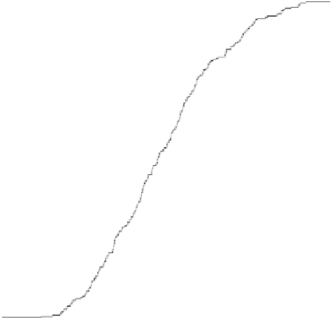
Femur Length (cm)
FIGURE 11.9
Comparison of the empirical cumulative density function for 250 simulated femoral lengths
(shown as a solid line step function) and the modeled cumulative density shown as a dashed line.
age-at-death for each individual given the estimated age-at-death structure and the “age
indicators.” We do this using Bayes' theorem as follows:
f
ðagejFL; lÞ
f
fðFLjageÞ
f
ðagejlÞ;
(11.20)
where the symbol
means proportional to rather than equal to. In Equation
11.20
the first
term on the right-hand side is the normal density for femur length given age (see
Figure 11.6
)
and the second term is from Equation
11.13
. Given femur length, we then search across Equa-
tion
11.20
to find the maximum density, which gives the best estimate of age for the indi-
vidual based on what we know about the age-at-death structure from the exponential
hazard model.
In
Figure 11.10
we have plotted these age estimates for femur lengths of 8
e
20 cm in 1 cm
increments and of 20
e
40 cm in 1 mm increments. We again use fractional polynomials to fit
a curve that allows us to quickly estimate age from any given femur length. The equation for
this curve is
age ¼ expð3:542 13:464=FL þ 1:748 logðFLÞÞ
and is shown as a solid
line. This line runs entirely through the plotted points. Another possibility is to solve the regres-
sion of femur length on age from the Maresh data (FL
¼ 3:6 þ 9:78
f
ag
p
) for age, in which
case we get
age ¼ 0:1355 0:0753 FL þ 0:0104 FL
2
, plotted as a second solid line in