Solid-Fuel Rocket Motor Efficiency Improvement Scheme - Novel Combustion Concepts for Sustainable Energy Development - page 542

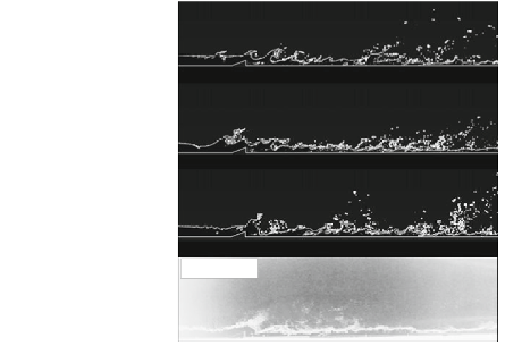
7.2 Simulation Result and Comparison

Figure 17 shows the VF of two-phase fl fluid of V air = 40 m/s at physical time at 4 s

after the both air and water start flowing from the left inlet of the channel domain by

computing with three different turbulence models: k-

fl

ε ˉ

, SST k- , and RSM. From

the figure it can be seen that the RSM demonstrates the highest rate of a breakup

behavior, SST k- model gives the least

amount of breakups among all the three turbulence models. It is difficult to tell
which turbulence model best matches the experimental due to the nature of transient
states; however, the experiment results will be clear after superposition treatment of
the ramp region. Treatment of the superposition of the turbulent for the ramp region
is given in the paragraph on the prehydraulic jump angle. Figure 18 summarizes the
averaged boundary length for all three different turbulence models, with boundary
length readings for k-

ˉ has medium rate of breakups, and k- ε

ε , SST k- ˉ , and RSM of 11.85, 12.79, and 12.87 m,

respectively. The RSM and SST k- ˉ show a similar boundary length value whereas

the k- model pro-

duces fewer breakups than the other two models. Standard deviations from the 260
time step of the respective models in the boundary length are 0.41, 0.40, and
0.61 m, as indicated by the error bars shown in Fig. 18 . Comparing the RSM and
SST k-

ε has the shortest boundary length which indicates that the k- ε

despite having a similar boundary length, the standard deviation of the
RSM is greater than the SST k-

ˉ

ˉ . This indicates that the two-phase fl flows of the

RSM run more unsteady than that of the SST k- ˉ . The k- ε model has a similar

standard deviation value with the SST k- ˉ

Fig. 17 Result of different
turbulence model and
experiment of V air = 40 m/s at
physical time T = 4.0 s
(Amano et al. 2014a , b )

k- ʵ

SST k- ˉ

RSM

Experiment