Game Development Reference
In-Depth Information
As we can see, it is less likely that the 25 events would be distributed over six
minutes than the usual five. Similarly, plugging
k
= 7 into the equation yields
10.4%; it is even
less
likely that 25 events would be spread over seven minutes. Each
value for
events oc-
curring in each discrete value of
k.
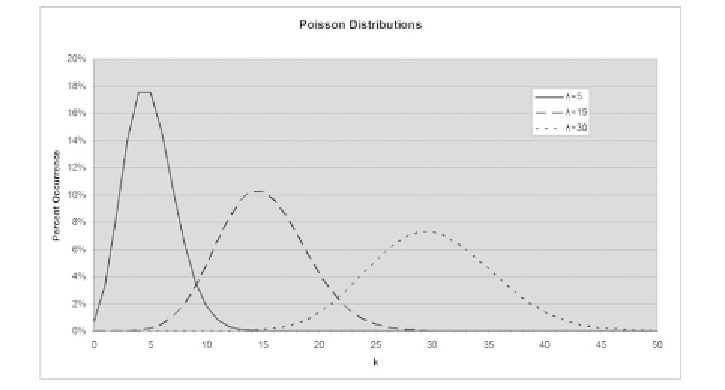
Figure 11.21 shows three examples for
λ
produces a distinct curve that expresses the probability of
λ
λ
values
of 5, 15, and 30.
FIGURE 11.21
If we change the value for
, the resulting curve spreads out
to account for the different probabilities.
λ
Another Use for Poisson
We can also use a Poisson distribution to model an event that happens once every
k
minutes instead of
times per minute. We use the same equation but simply
change our mindset. Referring again to Figure 11.21, we could use the curves shown
to represent events that happen every 5, 15, and 30 minutes. In this case, the prob-
abilities are the probability that the event happens during the specified time period.
For example, if we are expecting an event to happen
on average
every 15
minutes, (
λ
= 15), we would find that the actual recurrence of the event would be
distributed to values
around
15 minutes. It
may
occur at the 15-minute mark, but
it also may occur at 14 or 16 minutes. For that matter, it may occur at 5 or 30 min-
utes. The odds of those results are significantly less likely than 14 or 16, however.
We can observe this result easily by examining the associated curve.
The shapes of the curves are directly related to the value of
λ
. Loosely described,
the Poisson distribution takes an average interval and “fuzzies it up�? a bit. The longer
the interval, the more room for variation there is. That is, the longer the average
interval, the more possibility for “spread�? we can experience. For instance, if the
λ