Game Development Reference
In-Depth Information
In Figure 11.20, we show three similar parabolic curves being subtracted from
100 and arranged such that when
x
reaches 100,
y
reaches 0. The paths that the three
curves follow to get there are different, however. The shapes of the curves themselves
are different because the exponents are different: 2, 3, and 4. However, because the
results expand so rapidly, we needed to divide the equation by 100, 10,000, and
1,000,000, respectively. By doing that, we ensure that when
x =
100,
y
= 0.
Another useful, if slightly more esoteric, probability curve is the
Poisson distribution
.
Siméon-Denis Poisson originally developed it in 1838 as a way of expressing the
probability of events happening over time. Accordingly, we can use it in game AI to
generate events that occur at average intervals but without resorting to predictable
time periods. On the other hand, we are not limited to using the Poisson distribution
in connection with time-based events. We can benefit from using the unique prop-
erties of the Poisson distribution in other areas as well.
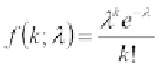
The formula for a Poisson distribution is:
The values in the equation are a little counter-intuitive at first and merit expla-
nation. The value
k
(the equivalent of
x
on the graph) represents the number of
occurrences of an event over a time period. The value
(lambda) is a positive, real
number equal to the expected number of occurrences over a given time period.
The familiar value
e
is the base of the natural logarithm (approximately 2.71828). The
result of the equation is the probability that
k
events will happen in that time period.
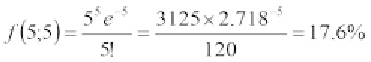
For example, if we know that an event happens five times in a minute on aver-
age (
λ
= 5), the Poisson distribution suggests that 17.6% of the time we can expect
it to occur exactly 25 times (5
λ
×
5) times in exactly five minutes.
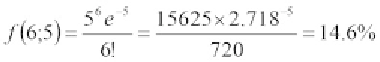
On the other hand, if we want to know how often we could expect it to happen
25 times (5
×
5) in
six
minutes, we would find: