Mathematical Functions - Behavioral Mathematics for Game AI - page 238

One of the advantages of the vertical range of the logistic function being [0...1]
is that it works very well as an expression of percentage. Despite being apparent on
the graph in Figure 10.6, it's worth noting that the function crosses the “50% mark�
at x = 0. If we think in those terms, we can see how the curve would be advanta-
geous in applications of psychology such as subjective utility functions.
For instance, if we were to say that we were “50% satisfied� with something
when it was “normal� (i.e., 0), we could then make the further observation that, as
that thing improved (i.e., x > 0), we would be more satisfied with it. Eventually, if
the improvement continued, we would approach a point where we were almost
100% satisfied with the object or action. Likewise, as the quality of the object or
action grew worse (i.e., x < 0), we would be less satisfied with it until such time as
we had almost 0% satisfaction.
In both cases, the further that the quality of that thing moved away from
“normal,� the less dramatic the effect is. This is reminiscent of marginal utility…
but in both directions away from the starting point. Unlike the root-based quadratic
equations that continued on to infinity in both directions, the asymptotic nature of
the logistic function provides the natural boundaries of 0% and 100%. After all, we
can't be less satisfied than “not at all� or more satisfied than “perfectly so.�
Also, because the vertical range of the curve is neatly defined, we can flip the
curve upside down quite easily by changing the formula to
Using the above formula, we find that the curve now starts near 1.0 when x <
0 and ends near 0.0 when x > 0.
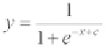
We can also shift the curve left or right in a fashion similar to the way we did
with other functions above. Using the same notation as before (the variable c ), our
new function would look like this:
Because the line extends infinitely in both directions, using the point where y
crosses the 0.5 mark is our best landmark. In the unshifted curve, when x = 0, y =
0.5. If we include a value for c , we know that y will cross the 0.5 mark where x = c .
As we noted before, the differences in value get insignificant outside the range of
about -6 to 6. Therefore, if we wanted the curve to start with x = 0, y = 0, we could
set c = 6. Accordingly, y would be within the same margin of 1.0 at about x = 12.