Database Reference
In-Depth Information
null
a
(7)
b
(6)
c
(7)
d
(6)
ab
(5)
ac
(5)
ad
(3)
bc
(4)
bd
(3)
cd
(4)
abc
(3)
abd
(2)
acd
(2)
bcd
(2)
abcd
(1)
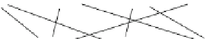
Fig. 10.1
An itemset lattice for the set of items
I
={
a
,
b
,
c
,
d
}
. Each node is a candidate itemset
with respect to transactions in Table
10.1
. For convenience, we include each itemset frequency.
Given
σ
=
0
.
5, tested itemsets are shaded
gray
and frequent ones have
bold borders
Table 10.1
Example
transactions with items from
the set
I
Tid
Items
1
a,b,c
={
a
,
b
,
c
,
d
}
2
a,b,c
3
a,b,d
4
a, b
5
a, c
6
a,c,d
7
c, d
8
b,c,d
9
a,b,c,d
10
d
2.2
Basic Mining Methodologies
Many sophisticated frequent itemset mining methods have been developed over the
years. Two core methodologies emerge from these methods for reducing compu-
tational cost. The first aims to prune the candidate frequent itemset search space,
while the second focuses on reducing the number of comparisons required to de-
termine itemset support. While we center our discussion on frequent itemsets, the
methodologies noted in this section have also been used in designing FSM and FGM
algorithms, which we describe in Sects.
5
and
6
, respectively.
2.2.1
Candidate Generation
A brute-force approach to determine frequent itemsets in a set of transactions is to
compute the support for every possible candidate itemset. Given the set of items
I
and a partial order with respect to the subset operator, one can denote all possible
candidate itemsets by an
itemset lattice
, in which nodes represent itemsets and edges
correspond to the subset relation. Figure
10.1
shows the itemset lattice containing
candidate itemsets for example transactions denoted in Table
10.1
. The brute-force