2.4
2.4.1
Adaptive quantizers. NICAM and ADPCM coders
We have already mentioned that if the probability density function (PDF) of the input is known one optimal quantizer can be computed for the signal. Linear or logarithmic quantizers are time-unvarying systems: their step sizes are fixed for the entire duration of the signal. Logarithmic quantizers (such as G.711) are an optimization that provides an SNR independent of the level of the signal.
It is also possible to adapt the quantizer dynamically to best match the instantaneous characteristics of the signal.
Many voice coders use dynamic quantization algorithms. The rules and types of adaptation used to encode the signal can be transmitted with the encoded signal (forward adaptive quantizers), but this is not required: backward adaptive quantizers use only the characteristics of the previously transmitted encoded signal to optimize the processing of the current sample(s), enabling the receiver to also compute the optimal adaptation that will be used for the next received encoded signal.
In addition, the optimal characteristics of the adaptive quantizer can be selected (or computed) for each sample, based on the characteristics of a group of contiguous samples (such a group is called a frame). A frame-based adaptation procedure is more efficient in terms of transmitted bitrate, especially when forward quantizer selection is used. The size of the frame must be selected carefully: if the size is too small there may be a large overhead for transmitting the scaling information, but if the block size is too large the quantizing steps may become inadequate for some portions of the frame, leading to large errors in the quantization process.
Figure 2.27 shows the principle of a forward adaptive quantizer and Figure 2.28 shows the principle of an inverse forward adaptive quantizer.
NICAM is an example of a coder using a forward adaptive quantizer (Figure 2.29). The NICAM (near-instantaneous companding and multiplexing) system is used to transmit the audio stereo signal digitally on analog TV channels using the PAL and SECAM TV color systems. The NICAM system transmits two stereo audio channels sampled at
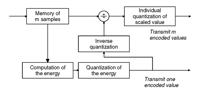
Figure 2.27 Principle of a forward adaptive quantizer.
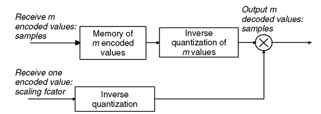
Figure 2.28 Principle of a forward adaptive inverse quantizer.
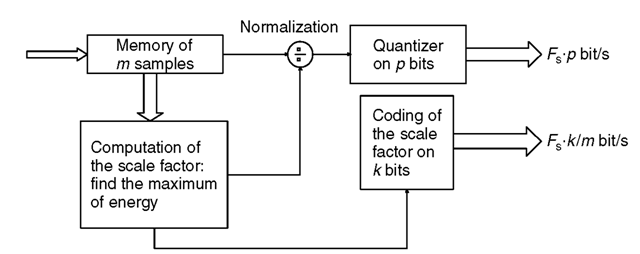
Figure 2.29 Near-instantaneous quantizer using: Fs • (p + k/m) bit/s.
32 kHz in a bitrate of 728 kbit/s. NICAM memorizes a buffer (the near-instantaneous characteristic …) of 32 samples and evaluates the mean power during this period of time, which is used to normalize the input samples. A fixed 10-bit logarithmic quantizer is then used on the normalized signal. The transmitted frame comprises the individual quantized samples, the scaling factor information, framing information, and some parity bits that protect the compressed audio signal against transmission errors.
It has been shown that, for the same subjective quality, the use of the quasi-instantaneous (32 samples) system requires 10.1 bits per sample compared with 11 bits per sample using a classical sample by sample logarithmic quantizer. There is a gain of 10% resulting from the use of block analysis and the forward ‘adaptive’ quantizer.
For backward adaptive quantizers, there is no need to transmit any information related to the scaling procedure; the mean power is estimated on the quantized signal and, therefore, the inverse quantizer can reconstruct this information exactly (Figures 2.30 and 2.31).
A very simple but efficient backward adaptive quantizer called ‘one-word memory’ is used in the ADPCM G.726 and G.727 ITU-T speech coders [A13]. A simple coefficient Mt depending only on the previous quantized sample determines the compression or expansion of the quantization steps for the next sample. If the quantizer has 4 bits (1 sign bit and 8 ranges of quantization), there are 8 Mt fixed coefficients (each implicitly associated with a quantizing range) insuring the compression or expansion of the quantizer. When large values are input to the quantizer, the multiplier value is greater than 1 and for small previous values the multiplier value is less than 1. This tends to force the
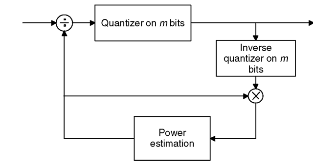
Figure 2.30 Principle of a backward adaptive quantizer.
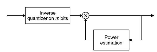
Figure 2.31 Principle of an m bit backward inverse quantizer.
adaptive quantizer to track the dynamics of the input signal (we can also consider that the previous measurement gave us some information on the probability density for the next sample, which we use to optimize the quantification). A fixed quantizer can be used and there is no need to transmit any scaling information to the decoder side (see Figures 2.32 and 2.33). Transmission errors will cause desynchronization of the coder and the decoder for a single sample.
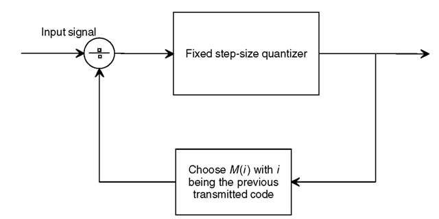
Figure 2.32 One-word memory adaptive quantizer.
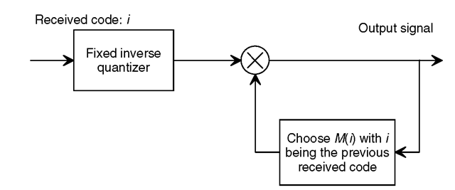
Figure 2.33 One-word memory adaptive inverse quantizer.
Table 2.7 Eight expansion coefficients attached to eight quantization ranges
| M0 | 0.969 |
| M1 | 0.974 |
| M2 | 0.985 |
| M3 | 1.006 |
| M4 | 1.042 |
| M5 | 1.101 |
| M6 | 1.208 |
| M7 | 1.449 |
Table 2.7 gives the Mt values for an eight-level quantizer (for each sign) optimized for exponential distribution.
The G.726 quantizer only needs to send 4 bits per sample (32 kbit/s), instead of 8 for G.711. G.726 is commonly used on many PSTN communication links when there is a need to reduce the transmitted bitrate.
2.4.2
Differential predictive quantization
In speech and audio signals, there is a strong correlation between the present sample and the previous one. The consequence is that if we subtract the previous sample from the present one, the variance of the difference signal will be lower than the variance of the original signal: it will require less bits to be quantized.
Unfortunately, we cannot directly use the exact previous sample value because it is inaccessible to the decoder. Instead, we must use the value of the previous sample as decoded by the receiver. In order to do this, the encoder relies on a ‘local decoder’ feedback loop which is common in speech and audio compression schemes. We have:
E(n) = X(n) — Xd(n — 1)
where Xd(n — 1) is the decoded value at time n — 1, and we transmit the quantized version of E(n), which is Q[E(n)].
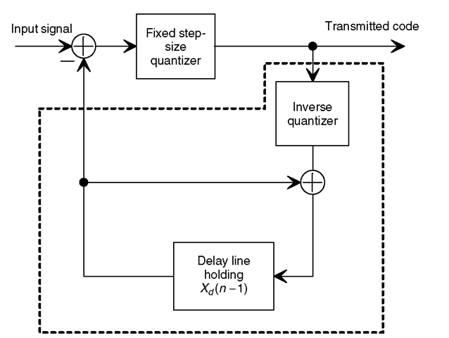
Figure 2.34 Principle of a differential quantizer (one-word memory prediction). The local decoder is in the dotted box and is identical to the distant decoder.
At the decoder side, we can compute the decoded value at time n:
![]()
Xd(n) approaches X(n), but has the small difference introduced by quantization noise: (Q—1[Q[E(n)]] — E(n)). If Q was ideal, then the noise signal would be zeroed.
Figure 2.34 illustrates the basic principle of a waveform speech or audio coder (called waveform because it tracks the temporal shape of the signal, as opposed to its frequency spectrum): all the concepts such as prediction or differential encoding are present.
The previous scheme is not a realistic one due to its sensibility to transmission errors: any transmission error will permanently desynchronize the decoder.
A more robust solution is to use a correlation coefficient:
![tmp42-58_thumb[1] tmp42-58_thumb[1]](http://lh3.ggpht.com/_X6JnoL0U4BY/S4PiyRUeexI/AAAAAAAATq4/hbhgenKYjO8/tmp4258_thumb1_thumb.png?imgmax=800)
where C1 is the correlation coefficient. A value below unity will decrease the influence of a transmission error over time.
Like all linear prediction schemes, this works only if there is some correlation in the input signal (i.e., it does not exhibit a flat frequency spectrum (white noise)). In the case of noise, there is no correlation between adjacent input samples. There is no chance to predict the future sample knowing the previous one. By contrast, speech and audio
signals, due to their production mode, exhibit a non-flat spectrum and consequently high correlation exists between samples.
This differential encoding method can be generalized by using more than one previous sample to build the predicted term and by using a dynamically computed correlation factor:
• In waveform or temporal coders working on a sample-by-sample basis, a temporal prediction of the signal is built from a linear combination of previous (decoded) samples. The coefficients are not transmitted; they are computed by a symmetrical procedure in the decoder.
• Vocoder or ABS speech coders filter the input signal by an inverse model based on correlation coefficients. It is the residual signal (output of the filter) which is encoded and transmitted with the modeling filter coefficients (called linear prediction coefficients, LPCs). LPC analysis is typically performed on a time frame of 10-30 ms at a sampling frequency of 8 kHz. This is a period of time where the speech signal can be considered as quasi-stationary.
In these algorithms, based on a history of more than one sample, the term Xd(n) is replaced by Xp(n), which is the value of the predicted signal based on previous samples:
![tmp42-59_thumb[2] tmp42-59_thumb[2]](http://lh5.ggpht.com/_X6JnoL0U4BY/S4PizuGH4dI/AAAAAAAATrA/e9S2NU_6uVQ/tmp4259_thumb2_thumb.png?imgmax=800)
As indicated in Figure 2.35, coefficients At can be fixed or ‘adaptive’ (i.e., computed for each new sample). When fixed, they are nonoptimal and derived from the average (if it really exists) frequency spectrum of the signal.
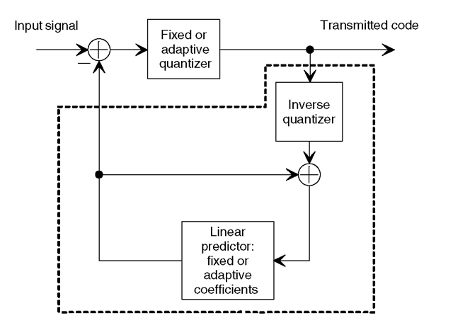
Figure 2.35 General principle of a differential (fixed or adaptive) coder. The local decoder is in the dotted box and is identical to the distant decoder.
Computation of the set of coefficients Ai in order to minimize quadratic error requires solving a set of linear equations [B2]. Even for a frame-by-frame analysis (such as for vocoder or ABS coders), this is a complex computational task which is out of reach of most real-time implementations. Many approximation algorithms have been developed to reduce computational complexity:
• For waveform coders, the set Ai, which is generally not transmitted, is continuously (on a sample-by-sample basis) adapted by the ‘stochastic gradient algorithm’ or by a simple ‘sign’ algorithm, where the absolute value of coefficients with the same sign as the error are reduced, and vice versa.
• For frequency or analysis by synthesis speech-coding schemes, the set Ai must be quantized and transmitted to the decoder side. The set of coefficients Ai or similar quantities modeling the short-term (10-30 ms) spectrum of the speech signal have to be computed. The direct inversion of the matrix obtained by expressing the minimization of quadratic errors is not used. More efficient algorithms have been studied and tuned to efficiently compute LPCs and to quantize them. Among them, the Levinson-Durbin algorithm and the Schur recursion are the most frequently used iterative methods to compute the Ai (Levinson-Durbin algorithm) or some partial coefficients called parcors (Schur recursion).
2.4.3
Long-term prediction for speech signal
Once a linear predictor (LPC, [B1]) has been used to filter the original speech signal, the correlation between adjacent samples is removed: the LPC filter 1 /A(z) models the average (short-term) spectrum of speech.
However, for voiced speech, the pitch introduces a long-term correlation. The fine structure of the speech spectrum is present in this residual signal. Due to pitch-induced quasi-periodicity, the residual signal still exhibits large variations. A pitch predictor can be used to remove the long-term correlation remaining in the residual signal. The simplest form of this pitch predictor filter (called the long term predictor (LTP) filter)is B(z) = 1 — jz—M,where M is the pitch period and jj a scalar gain. This filter subtracts from the current speech sample the value of a previous sample (at a distance of M samples) with a scaling factor of j . This procedure reduces the quasi-periodic behavior of the residual signal. A more generalized form of this LTP filter is B(z) = 1 —J2i 5iz—M—l, called a multi-tap LTP filter.
In speech processing and coding, one of the main issues is to find the parameters of this LTP filter: the gain and lag values (jj and M). These coefficients can be computed by evaluating the inter-correlation between frames of speech with different lag values and to find the maximum of these inter-correlation values; each maximum determines a lag value. Then the gain can be obtained by the normalization procedure (division of the power of the frame by the maximum inter-correlation found; sometimes an LTP gain of greater than unity can be found). This procedure is known as an open-loop search procedure as opposed to the closed-loop search found in some advanced CELP coders (adaptive codetopic for long-term prediction).
Very often, since the frame length of speech coders is generally in the range 160-240 samples and the number of samples between two pitch periods is between 20 and 140, an LTP analysis is done on a subframe basis; this is also due to the fact that the pitch lag varies faster than the vocal tract (LPC filter). Moreover, the pitch lag may be not exactly equal to an entire number of samples, leading to the concept of fractional lags used in the LTP filter. The procedure to find this fractional lag must upsample the signal to be analyzed in order to find a fractional lag; for example, upsampling by a factor of 8 allows us to find a lag with a precision equal to one-eighth of the sampling period (generally for speech, 125 (is). This fractional lag LTP is much more time-consuming, but it significantly improves the quality of decoded speech.
2.4.4
Vector quantization
Up to now, we have focused on sample-by-sample quantizers. With sample-by-sample, or scalar, quantization, each sample is mapped or rounded off to one discrete element of the codetopic. This can be optimized by forming vectors of samples (or other quantities such as LPC or LSP coefficients) which can be quantized jointly in a single operation. Vector quantization is one of the most powerful tools used in modern speech and audio coders. In vector quantization, a block of M samples (or other items such as linear predictive coefficients) forms a vector that is mapped at predetermined points in M-dimensional space and portioned into cells; Figure 2.36 shows the case of bidimensional space.
For scalar quantization, quantization noise is added to each sample to be encoded and decoded; on the other hand, for vector quantization, the noise is concentrated around
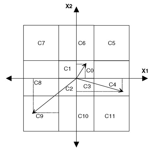
Figure 2.36 Vector quantization. Two-dimensional space for a vector quantizer Vectors of components X1 and X2 are localized in cells C0 to C11; the index of the cell is transmitted at the decoder.
the selected vector and correlated for all components. Generally, vector quantization is more efficient than scalar quantization because the codetopic can be optimized to use this correlation. For example, in vocoders or source speech coders, such as the LPC 10, independent scalar quantization of the ten LPC coefficients requires about 50 bits per frame (20-30 ms), but vector quantization needs only 25 bits per frame for the same subjective and perceived quality.
This is a significant improvement, but the counterpart is that vector quantization requires much more processing power and is also more sensitive to transmission errors than scalar quantization: an error on one decoded vector impacts all the individual elements of the vector.
There are several types of vector quantization procedures, such as binary, gain shape, split, etc.: in each case the design and optimization of the codetopic is of prime importance. Optimizing space partitioning and finding the best vector representatives requires a very large database so that the codettopic can be optimized. Distortion measures correlated with human perception and some subjective tests are sometimes required to choose the best codetopic.
2.4.5
Entropy coding
This technique is not specific to speech and audio coders, it is also used for most video coders and fax, as well as many file compression tools. The principle of entropy encoding is to map the parameters to be transmitted (e.g., a bit pattern) to code words of variable length, and to use shorter (with a minimum number of bits) code words to represent more frequently transmitted parameter values and longer code words for the least used. Huffman codes and RLC (running length code) are some representatives of such codes.
Huffman coding [A21] represents an object with a number of bits that is smaller for objects with larger probabilities. The algorithm builds a binary tree iteratively by first assembling the two objects with the lowest probabilities m1 and &>2 in a node associated with weight m1 + &>2. The object with the smallest probability m1 is located to the left of the node. The new node with weight m1 + co2 is added to the collection of objects and the algorithm is restarted (Figure 2.37).
Such an entropy-coding scheme can be placed after a classical speech or audio coder on the bitstream to be transmitted. No additional framing information is required in the encoded bitstream (prefix condition code).
