APPLICATIONS OF THE BINOMIAL DISTRIBUTION TO EVALUATE CALL OPTIONS
In this topic, we show how the binomial distribution is combined with some basic finance concepts to generate a model for determining the price of stock options.
What is an Option?
In the most basic sense, an option is a contract conveying the right to buy or sell a designated security at a stipulated price. The contract normally expires at a predetermined date. The most important aspect of an option contract is that the purchaser is under no obligation to buy; it is, indeed, an ”option.” This attribute of an option contract distinguishes it from other financial contracts. For instance, whereas the holder of an option may let his or her claim expire unused if he or she so desires, other financial contracts (such as futures and forward contracts) obligate their parties to fulfill certain conditions.
A call option gives its owner the right to buy the underlying security, a put option the right to sell. The price at which the stock can be bought (for a call option) or sold (for a put option) is known as the exercise price.
The Simple Binomial Option Pricing Model
Before discussing the binomial option model, we must recognize its two major underlying assumptions. First, the binomial approach assumes that trading takes place in discrete time, that is, on a period-by-period basis. Second, it is assumed that the stock price (the price of the underlying asset) can take on only two possible values each period; it can go up or go down.
Say we have a stock whose current price per share S can advance or decline during the next period by a factor of either u (up) or d (down). This price either will increase by the proportion u —1>0 or will decrease by the proportion 1—d, 0< d<1. Therefore, the value S in the next period will be either uS or dS. Next, suppose that a call option exists on this stock with a current price per share of C and an exercise price per share of X and that the option has one period left to maturity. This option’s value at expiration is determined by the price of its underlying stock and the exercise price X. The value is either

Why is the call worth Max (0, uS — X) if the stock price us uS? The option holder is not obliged to purchase the stock at the exercise price of X, so she or he will exercise the option only when it is beneficial to do so. This means the option can never have a negative value. When is it beneficial for the option holder to exercise the option? When the price per share of the stock is greater than the price per share at which he or she can purchase the stock by using the option, which is the exercise price, X. Thus if the stock price uS exceeds the exercise price X, the investor can exercise the option and buy the stock. Then he or she can immediately sell it for uS, making a profit of uSX (ignoring commission). Likewise, if the stock price declines to dS, the call is worth Max (0, dS – X).
Also for the moment, we will assume that the risk-free interest rate for both borrowing and lending is equal to r percent over the one time period and that the exercise price of the option is equal to X.
To intuitively grasp the underlying concept of option pricing, we must set up a risk-free portfolio – a combination of assets that produces the same return in every state of the world over our chosen investment horizon. The investment horizon is assumed to be one period (the duration of this period can be any length of time, such as an hour, a day, a week, etc.). To do this, we buy h share of the stock and sell the call option at its current price of C. Moreover, we choose the value of h such that our portfolio will yield the same payoff whether the stock goes up or down.

By solving for h, we can obtain the number of shares of stock we should buy for each call option we sell.

Here h is called the hedge ratio. Because our portfolio yields the same return under either of the two possible states for the stock, it is without risk and therefore should yield the risk-free rate of return, r percent, which is equal to the risk-free borrowing and lending rate, the condition must be true; otherwise, it would be possible to earn a risk-free profit without using any money. Therefore, the ending portfolio value must be equal to (1 + r) times the beginning portfolio value, hS – C.

Note that S and C represent the beginning values of the stock price and the option price, respectively.
Setting R = 1 + r, rearranging to solve for C, and using the value of h from Equation (G4), we get

where d < r < u. To simplify this equation, we set

Thus we get the option’s value with one period to expiration

This is the binomial call option valuation formula in its most basic form. In other words, this is the binomial valuation formula with one period to expiration of the option.
To illustrate the model’s qualities, let’s plug in the following values, while assuming the option has one period to expiration. Let
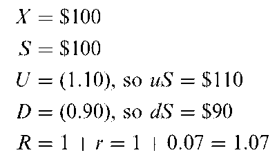
Table G.1. Possible Option Value at Maturity
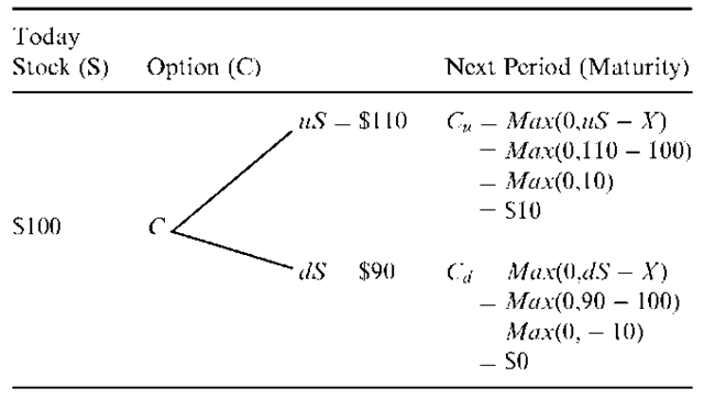
First we need to determine the two possible option values at maturity, as indicated in Table G.1.
Next we calculate the value of p as indicated in Equation (G7).

Solving the binomial valuation equation as indicated in Equation (G8), we get
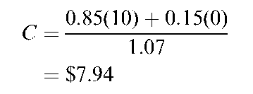
The correct value for this particular call option today, under the specified conditions, is $7.94. If the call option does not sell for $7.94, it will be possible to earn arbitrage profits. That is, it will be possible for the investor to earn a risk-free profit while using none of his or her own money. Clearly, this type of opportunity cannot continue to exist indefinitely.
The Generalized Binomial Option Pricing Model
Suppose we are interested in the case where there is more than one period until the option expires. We can extend the one-period binomial model to consideration of two or more periods.
Because we are assuming that the stock follows a binomial process, from one period to the next it can only go up by a factor of u or go down by a factor of d. After one period the stock’s price is either uS or dS. Between the first and second periods, the stock’s price can once again go up by u or down by d, so the possible prices for the stock two periods from now are uuS, udS, and ddS. This process is demonstrated in tree diagram (Figure G.1) given in Example G.1 later in this topic.
Note that the option’s price at expiration, two periods from now, is a function of the same relationship that determined its expiration price in the
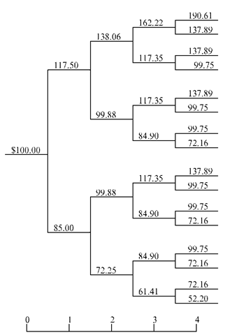
Figure G.1. Price Path of Underlying Stock Source: Rendelman, R.J., Jr., and Bartter, B.J. (1979). “Two-State Option Pricing,” Journal of Finance 34 (December), 1906.
one-period model, more specifically, the call option’s maturity value is always

where T designated the maturity date of the option.
To derive the option’s price with two periods to go (T = 2), it is helpful as an intermediate step to derive the value of Cu and Cd with one period to expiration when the stock price is either uS or dS, respectively.

Equation (G10) tells us that if the value of the option after one period is Cu, the option will be worth either Cuu (if the stock price goes up) or Cud (if stock price goes down) after one more period (at its expiration date). Similarly, Equation (G11) shows that the value of the option is Cd after one period, the option will be worth either Cdu or Cdd at the end of the second period. Replacing Cu and Cd in Equation (G8) with their expressions in Equations (G10) and (G11), respectively, we can simplify the resulting equation to yield the two-period equivalent of the one-period binomial pricing formula, which is

In Equation (G12), we used the fact that Cud = Cdu because the price will be the same in either case.
We know the values of the parameters S and X. If we assume that R, u, and d will remain constant over time, the possible maturity values for the option can be determined exactly. Thus deriving the option’s fair value with two periods to maturity is a relatively simple process of working backwards from the possible maturity values.
Using this same procedure of going from a one-period model to a two-period model, we can extend the binomial approach to its more generalized form, with n periods maturity

To actually get this form of the binomial model, we could extend the two-period model to three periods, then from three periods to four periods, and so on. Equation (G13) would be the result of these efforts. To show how Equation (G13) can be used to assess a call option’s value, we modify the example as follows: S = $100, X = $100, R = 1.07, n = 3, u = 1.1 and d = 0.90.
First we calculate the value of p from Equation (G7) as 0.85, so 1 — p is 0.15. Next we calculate the four possible ending values for the call option after three periods in terms of Max[0, ukdn—kS — X].
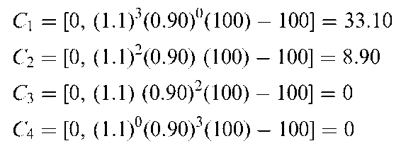
Now we insert these numbers (C1, C2, C3, and C4) into the model and sum the terms.
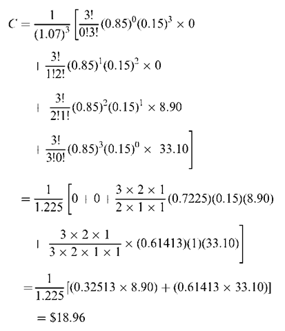
As this example suggests, working out a multiple-period problem by hand with this formula can become laborious as the number of periods increases. Fortunately, programming this model into a computer is not too difficult.
Now let’s derive a binomial option pricing model in terms of the cumulative binomial density function. As a first step, we can rewrite Equation (G13) as
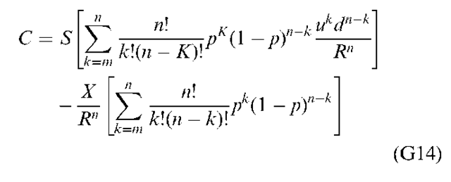
This formula is identical to Equation (G13) except that we have removed the Max operator. In order to remove the Max operator, we need to make ukdn—kS — X positive, which we can do by changing the counter in the summation from k = 0 to k = m. What is m? It is the minimum number of upward stock movements necessary for the option to terminate ”in the money” (that is, ukdn—kS — X > 0). How can we interpret Equation (G14)? Consider the second term in brackets; it is just a cumulative binomial distribution with parameters of n and p. Likewise, via a small algebraic manipulation we can show that the first term in the brackets is also a cumulative binomial distribution. This can be done by defining P’ = (u/R)p and 1 — P’ = (d/R)(1 — p). Thus

Therefore the first term in brackets is also a cumulative binomial distribution with parameters of n and p’. Using Equation (G10) in the text, we can write the binomial call option model as
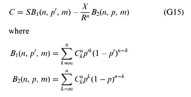
and m is the minimum amount of time the stock has to go up for the investor to finish in the money (that is, for the stock price to become larger than the exercise price).
In this topic, we showed that by employing the definition of a call option and by making some simplifying assumptions, we could use the binomial distribution to find the value of a call option. In the next chapter, we will show how the binomial distribution is related to the normal distribution and how this relationship can be used to derive one of the most famous valuation equations in finance, the Black-Scholes option pricing model.
Example G.1
A Decision Tree Approach to Analyzing Future Stock Price
By making some simplifying assumptions about how a stock’s price can change from one period to the next, it is possible to forecast the future price of the stock by means of a decision tree. To illustrate this point, let’s consider the following example.
Suppose the price of Company A’s stock is currently $100. Now let’s assume that from one period to the next, the stock can go up by 17.5 percent or go down by 15 percent. In addition, let us assume that there is a 50 percent chance that the stock will go up and a 50 percent chance that the stock will go down. It is also assumed that the price movement of a stock (or of the stock market) today is completely independent of its movement in the past; in other words, the price will rise or fall today by a random amount. A sequence of these random increases and decreases is known as a random walk.
Given this information, we can lay out the paths that the stock’s price may take. Figure G.1 shows the possible stock prices for company A for four periods.
Note that in period 1 there are two possible outcomes: the stock can go up in value by 17.5 percent to $117.50 or down by 15 percent to $85.00. In period 2 there are four possible outcomes. If the stock went up in the first period, it can go up again to $138.06 or down in the second period to $99.88. Likewise, if the stock went down in the first period, it can go down again to $72.25 or up in the second period to $99.88. Using the same argument, we can trace the path of the stock’s price for all four periods.
If we are interested in forecasting the stock’s price at the end of period 4, we can find the average price of the stock for the 16 possible outcomes that can occur in period 4.
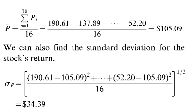
P and sP can be used to predict the future price of stock A.
