Introduction
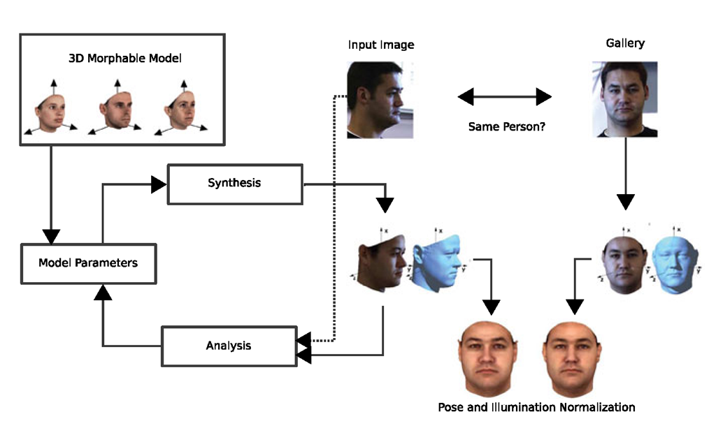
Our approach is based on an analysis by synthesis framework. In this framework, an input image is analyzed by searching for the parameters of a generative model such that the generated image is as similar as possible to the input image. The parameters are then used for high-level tasks such as identification.
To be applicable to all input face images, a good model must be able to generate all possible face images. Face images vary widely with respect to the imaging conditions (illumination and the position of the camera relative to the face, called pose) and with respect to the identity and the expression of the face. A generative model must not only allow for these variations but must also separate the sources of variation such that e.g. the identity can be determined regardless of pose, illumination or expression.
In this topic, we present the Morphable Model, a three-dimensional (3D) representation that enables the accurate modeling of any illumination and pose as well as the separation of these variations from the rest (identity and expression). The Morphable Model is a generative model consisting of a linear 3D shape and appearance model plus an imaging model, which maps the 3D surface onto an image. The 3D shape and appearance are modeled by taking linear combinations of a training set of example faces. We show that linear combinations yield a realistic face only if the set of example faces is in correspondence. A good generative model should accurately distinguish faces from nonfaces. This is encoded in the probability distribution over the model parameters, which assigns a high probability to faces and a low probability to nonfaces. The distribution is learned together with the shape and appearance space from the training data.
Based on these principles, we detail the construction of a 3D Morphable Face Model in Sect. 6.2. The main step of model construction is to build the correspondences of a set of 3D face scans. Such models have become a well-established technology which is able to perform various tasks, not only face recognition, but also face image analysis [6] (e.g., estimating the 3D shape from a single photograph), expression transfer from one photograph to another [10, 46], animation of faces [10], training of feature detectors [22, 24], and stimuli generation for psychological experiments [29] to name a few. The power of these models comes at the cost of an expensive and tedious construction process, which has led the scientific community often to focus on more easily constructed but less powerful models. Recently, a complete 3D Morphable Face Model built from 3D face scans, the Basel Face Model (BFM), was made available to the public (faces.cs.unibas.ch) [34]. An alternative approach to construct a 3D Morphable Model is to generate the model directly from a video sequence [12] using nonrigid structure from motion. While this requires far less manual intervention, it also results in a less detailed and inaccurate model.
With a good generative face model, we are half the way to a face recognition system. The remaining part of the system is the face analysis algorithm (the fitting algorithm). The fitting algorithm finds the parameters of the model that generate an image which is as close as possible to the input image. In this topic, we focus on fitting the model to a single image. We detail two fitting algorithms in Sect. 6.4.
Based on these two fitting algorithms, identification results are presented in Sect. 6.5 for face images varying in illumination and pose, as well as for 3D face scans. The fitting methods presented here are energy minimization methods, a different class of fitting methods are regression based, and try to learn a correspondence between appearance and model coefficients. For 2D Models, [20] proposed to learn a linear regression mapping the residual between a current estimate and the final fit, and [27] proposed to use a support vector regression on Haar features of the image to directly predict 6 coefficients of a 2D mouth model from 12 Haar features of mouth images.
Three-Dimensional Representation
Each individual face can generate a variety of images when seen from different viewpoints, under different illumination and with different expressions. This huge diversity of face images makes their analysis difficult. In addition to the general differences between individual faces, the appearance variations in images of a single faces can be separated into the following four sources.
• Pose changes can result in dramatic changes in images. Due to self-occlusions different parts of the object become visible or invisible. Additionally, the parts seen in two views change their spatial configuration relative to each other.
• Illumination changes influence the appearance of a face even if the pose of the face is fixed. The distribution of light sources around a face changes the brightness distribution in the image, the locations of attached shadows, and specular reflections. Additionally, cast shadows can generate prominent contours in facial images.
• Facial expressions are another source of variations in images. Only a few facial landmarks that are directly coupled with the bony structure of the skull, such as the corners of the eye or the position of the earlobes, are constant in a face. Most other features can change their spatial configuration or position via articulation of the jaw or muscle action (e.g., moving eyebrows, lips, or cheeks).
• On a longer timescale faces change because of aging, change of hairstyle, and the use of makeup or accessories.
The isolation and explicit description of these sources of variations must be the ultimate goal of a face analysis system. For example, it is desirable that the parameters that code the identity of a person are not perturbed by a modification of pose. In an analysis by synthesis framework, this implies that the face model must account for each of these variations independently by explicit parameters.
We need a generative model which is a concise description of the observed phenomena. The image of a face is generated according to the laws of physics which describe the interaction of light with the face surface and the camera. The parameters for pose and illumination can therefore be described most concisely when modeling the face as a 3D surface. A concise description of the variability of human faces on the other hand can not be derived from physics. We therefore describe the variations in 3D shape and albedo of human faces with parameters learned from examples.
Correspondence-Based Representation
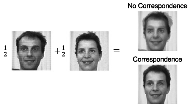
Early face recognition techniques used a purely appearance-based representation for face analysis. In an appearance based representation such as eigenfaces [40, 43] and their generalized version from [33], it is assumed that face images behave like a vector space, that is, the result of linearly combining face images yields a new face image. These techniques have been demonstrated to be successful when applied to images of a set of very different objects, or when the viewpoint and lighting conditions are close to constant and the image resolution is relatively low. These limitations come from the wrong assumption that face images form a vector space. We illustrate this in Fig. 6.1 by showing that already the mean of two face images has double edges and is no longer a face. Even though face images do not form a vector space, faces do form a vector space when using the correct representation. The artifacts visible in the averaged face in Fig. 6.1 come from the fact that pixels from different positions on the two faces, have been combined to generate the new pixel value. In an image, face shape and appearance are mixed. If one separates the face shape and the face appearance by establishing correspondence between the input images, then the faces can be linearly combined, see Fig. 6.1 lower right.
Separating face shape and face appearance means that one chooses an underlying parametrization of a face (the face domain), independently from the images. The shape of a face in an image is then expressed as the correspondence between the face domain and the image, and the appearance of a face by the image mapped back into the face domain. Within the face domain, the color and shape of different faces can be linearly combined to yield new faces. In addition, one also separates the shape into a local deformation and a camera model, which positions the face inside the target image. When discretizing the face domain, we can express face shape and appearance by a vectors of shape displacements and color. The combination of the shape and appearance vector spaces is called face subspace.
A separation of shape and appearance—also called an object center representation—has been proposed by multiple authors [5, 15, 23, 28, 45]; for a review see Beymer and Poggio [4]. It should be noted that some of these approaches do not use the correspondence between points which are actually corresponding on the underlying faces: The methods using 2D face models, for example, Lanitis et al. [28], often put into correspondence the 2D occluding contour, which corresponds to different positions on the face depending on the pose. In contrast, our approach uses the 3D shape of faces as the face domain and establishes the true correspondences between the underlying faces.
Face Statistics
In the previous section, we explained that correspondences enable the generation of new faces as a linear combination of training faces. However, the coefficients of the linear combination do not have a uniform distribution. This distribution is learned from example faces using the currently widely accepted assumption that the face subspace is Gaussian. Under this assumption, PCA is used to learn a probability model of faces that is used as prior probability at the analysis step (see Sect. 6.4.1). More details about the face statistics of our model are given in Sects. 6.2.3 and 6.2.4.
Fig. 6.1 Computing the average of two face images using different image representations. No correspondence information is used (top right) and using correspondence (bottom right)
3D Morphable Model Construction
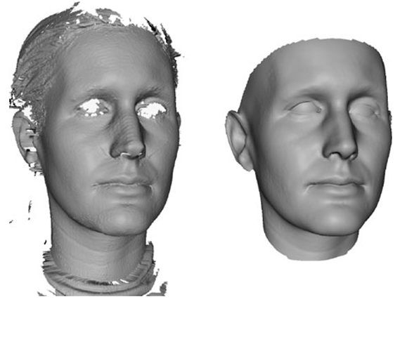
The construction of a 3D Morphable Model requires a set of example 3D face scans with a large variety. The results presented in this section were obtained with a Mor-phable Model constructed with 200 scans (100 female and 100 male), most of them Europeans. This Morphable Model has been made publicly available (Basel Face Model: faces.cs.unibas.ch [34]) and can be freely used for noncommercial purposes. The constructions are performed in three steps: First, the scans are preprocessed. This semiautomatic step aims to remove the scanning artifacts and to select the part of the head that is to be modeled (from one ear to the other and from the neck to the forehead). In the second step, the correspondences are computed between each of the scans and a reference face mesh (see Fig. 6.2 for an example). The registered faces scans are then aligned using Generalized Procrustes Analysis such that they do not contain a global rigid transformation. Then a principal component analysis is performed to estimate the statistics of the 3D shape and color of the faces.
3D Face Scanning
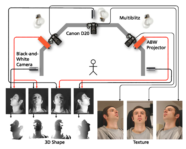
For 3D face scanning it is important to have not only high accuracy but also a short acquisition time, such that the scans are not disrupted by involuntary motions, and the scanning of facial expressions is possible. We decided to use a coded light system (Fig. 6.3) because of its high accuracy and short acquisition time (~1 s) compared to laser scanners (~15 s as used in [6]).
The system captures the face shape from ear to ear (Fig. 6.2, left) and takes three color photographs. The 3D shape of the eyes and hair cannot be captured with our system, due to their reflection properties.
Fig. 6.2 The registration of the original scan (left) establishes a common parametrization and fills in missing data (right)
Fig. 6.3 3D face scanning device developed by ABW-3D. The system consists of two structured light projectors, three gray level cameras for the shape, three 8 mega pixel SLR cameras and three studio flash lights
Registration
To establish correspondence, there exist two different approaches: mesh-based algorithms and algorithms modeling the continuous surface using variational techniques. Variational methods are mostly used in medical image analysis (e.g., [17, 25, 30]) where the input is typically already a voxelized volume. For 3D face surfaces, mesh-based algorithms are mostly used (e.g., [1, 3]). Here, we use a nonrigid ICP method similar to [1], that is applied in the 3D domain on triangulated meshes. It progressively deforms a template towards the measured surface. The correlated correspondence algorithm [3] is a very different approach to range scan registrations that is applicable to both faces and bodies.
The nonrigid ICP algorithm works as follows: First, for each vertex of the template a corresponding target point in the scanned surface is determined. This is done by searching for the point in the scan which is closest to the vertex of the deformed template, has a compatible normal and does not lie on the border of the scan. The template is then deformed such that the distance between the deformed template and the correspondence points is minimized subject to a regularization which prohibits strong deformations, bringing the template closer to the surface. We use a regularization which minimizes the second derivative of the deformation measured along the template surface. By starting with a strong regularization, we first recover the global deformations. The regularization is then lowered, allowing progressively more local deformations.
The steps of the algorithm are as follows:
Algorithm 6.1: Nonrigid ICP registration
The template shape is created in a bootstrapping process, starting with a manually created head model with an optimized mesh using discrete conformal mappings [26]. It is first registered to the target scans, then the average over all registrations is used as a new template. This process is iterated a few times involving further manual corrections to achieve a good template shape. The template defines the parametrization of the model and it is used to fill in holes in the measurement. Wherever no correspondences are found, the deformation is extended smoothly along the template surface by the regularization. This fills in unknown regions with the deformed template shape.
The regularization uses a discrete approximation of the second derivative of the deformation field, which is calculated by finite differencing between groups of three neighboring vertices. The cost function in [1] uses first order finite differences, and can be adapted in a straightforward way to second order finite differences.
The scanner produces four partially overlapping measurements (shells) of the target surface (Fig. 6.3), which have to be blended. This blending is done during registration by determining the closest point as a weighted average of the closest points of all shells. The weighting is performed with a reliability value computed from the distance between the scan border and the angle between surface normal and camera direction.
The registration method so far is purely shape based, but we have included additional cues from our scanning system. Some face features like the outline of the lips and the eyebrows are purely texture based, and do not have corresponding shape variations. To align these features in the model, we semi-automatically label the outlines of the lips, eyes and eyebrows in the texture photographs, and constrain the corresponding vertices of the deformed template to lie in the extrusion surfaces defined by the back-projection of these lines. Additionally, as the shape of the ears is not correctly measured by the scanner, we mark the outline of the ears in the images to get at least the overall shape of the ears right.
To initialize the registration, some landmarks are used. The weighting of the landmark term is reduced to zero during the optimization, as these points cannot be marked as accurately as the line landmarks. In a preprocessing step, the scanned data is smoothed using mean curvature flow [16] on the depth images.
Since the shape of the eyeballs is not correctly measured by the scanner, we replace them by spheres fit to the vertices of the eyes. This is done after the registration in a post-processing step.
The projection of each pixel of the high resolution texture photos onto the geometry is calculated, resulting in three overlapping texture maps. These are blended based on the distance from the visible boundaries and the orientation of the normal relative to the viewing direction. Hair is manually removed from the resulting texture, and the missing data is filled in by a diffusion process.
PCA Subspace
Section 6.1.2 introduced the idea of a face subspace, wherein all faces are con-structable by a generative model lie. We now detail the construction of the face subspace for a 3D Morphable Model. The face subspace is constructed by putting a set of M example 3D face scans into correspondence with a reference face. This introduces a consistent labeling of all Nv 3D vertices across all the scans: each registered face is represented by a triangular mesh with Nv = 53490 vertices. Each vertex j consists of a 3D point with an associated per vertex color
 Due to the correspondence, the mesh topology is the same for each face.
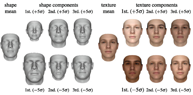
Fig. 6.4 The mean together with the first three principle components of the shape (left) and texture (right) PCA model. Shown is the mean shape resp. texture plus/minus five standard deviations σ
These 3D meshes are a discretization of the continuous underlying face domain. Each shape or texture can be represented as a 3 x Nv matrix
We can now take linear combinations of the M example faces to produce new faces corresponding to new individuals.
While these linear combinations do contain all new faces, they also contain non faces. All convex combinations of faces are again faces, and also vectors close to the convex area spanned by the examples are faces, but points far away from the convex area correspond to shapes which are very unlikely faces. When for example setting all but one coefficient to 100, we get a face which is 100 times as big as the example face. It is very unlikely that we will encounter such a face in the real world. This argument shows, that each coefficient vector needs an assigned probability of describing a face. We model this probability by a Gaussian distribution with a block diagonal matrix, which assumes that shape and texture are decorrelated. Assuming a Gaussian allows us to approximate the face subspace with a smaller set of orthogonal basis vectors, which are computed with Principal Component Analysis (PCA) from the training examples.
Principal component analysis (PCA) is a statistical tool that transforms the space such that the covariance matrix is diagonal (i.e., it decorrelates the data). We describe the application of PCA to shapes; its application to textures is straightforward. The resulting model is shown in Fig. 6.4. After subtracting their average, S, the exemplars are arranged in a data matrix A and the eigenvectors of its covariance matrix C are computed using the singular value decomposition [37] of A.
The component vec(S) vectorizes S by stacking its columns. The M columns of the orthogonal matrix U are the eigenvectors of the covariance matrix C, and
 are its eigenvalues, where the Xi are the elements of the diagonal matrix W, arranged in decreasing order. Let us denote Uv-, the column i of U, and the principal component i, reshaped into a 3 x Nv matrix, by
 The notation
 [31] folds the m x 1 vector a into an n x (m/n) matrix.
Now, instead of describing a novel shape and texture as a linear combination of examples, as in (6.2), we express them as a linear combination of Ns shape and Nt texture principal components.
The advantage of this formulation is that the probabilities associated with a shape and texture are readily available.
