Face Alignment Models (Face Image Modeling and Representation) (Face Recognition) Part 2

Statistical Models of Texture

Though the shape of a face may give a weak indication of identity, the texture of the face provides a far stronger cue for recognition. We therefore apply similar techniques to those used to build a shape model in order to build a model of texture, given a set of training images. Fitting the texture model to new image data then summarising the properties of the underlying face (including its identity) through the texture model parameters.

Aligning Sets of Textures

Given a set of training images of faces that are coarsely-aligned (e.g., with respect to similarity transformations only), it has been shown that a linear subspace-based face model [34] provides a useful representation for recognition [58]. However, this coarse alignment does not compensate for nonrigid variation in shape due to identity, pose or expression. As a result, corresponding pixels over the set of training images actually originate from different points on the face (or possibly even the background) and spurious texture variation creeps into the model, reducing recognition performance [19].

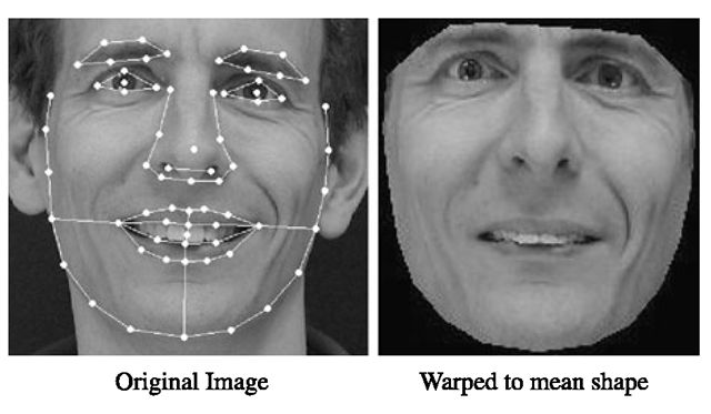
To address this problem, we use the correspondences between facial features (e.g., eyes, nose and mouth) over the set of labelled training images to define an approximate correspondence between the pixels in the underlying image [4, 18]. In particular, we apply a continuous deformation—such as an interpolating spline or a piece-wise affine warp using a triangulation of the region—to warp each training image so that its feature points match a reference shape (typically the mean shape). The intensity information is then sampled from the shape-normalised image over the region covered by the mean shape (Fig. 5.3) to form a texture vector, gm. Since gim is defined in the normalised shape frame, it has a fixed number of pixels, npixels, that is independent of the size of the object in the target image.

This nonlinear sampling (Algorithm 5.4) applies a geometric alignment of the textures, ensuring that corresponding elements over the set of texture vectors represent corresponding points on the face so that computed image statistics are meaningful. As in the case of the shape model, however, we want our texture model to represent only those changes that cannot be explained by a global transformation (e.g., due to changes in brightness and contrast). We therefore apply a photometric alignment of the texture samples before computing the image statistics that will define our texture model.

Fig. 5.3 Example of face warped to the mean shape. Although the main shape variations due to smiling have been removed, there is considerable texture difference from a purely neutral face

Algorithm 5.4: Texture sampling

More specifically, we express a texture in the image frame as a 1D affine transformation, Tu(·), of the corresponding model texture, g, such that

whereis a vector of parameters corresponding to contrast and brightness, and u = 0 gives the identity transformation. Unlike shape normalisation, this transformation is linear and we can find a closed-form solution for parameters to give the sampled vector, g^, zero sum and unit variance is the number of elements in the vectors. The normalised texture vector in the model frame is then given by the inverse transformation,:

where npixels is the number of elements in the vectors. The normalised texture vector in the model frame is then given by the inverse transformation,

For colour images, each plane can be normalised separately though we have found that grey-scale models are able to generalise to unseen images more effectively than colour models.

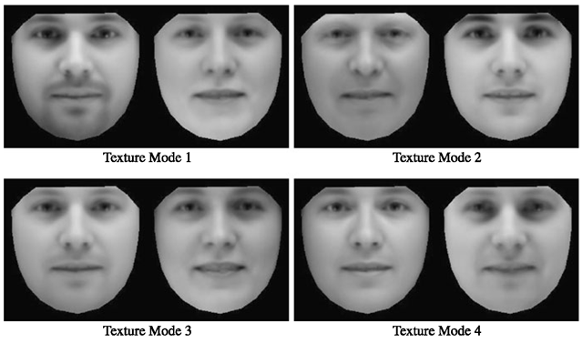
Fig. 5.4 Four modes of a face texture model built from 400 images (including neutral, smiling, frowning and surprised expressions) of 100 different individuals with around 20000 pixels per example. Texture parameters have been varied by ±2 standard deviations from the mean

Linear Models of Texture Variation

Once we have compensated for the effects of brightness and contrast, we apply PCA to the set of normalised texture vectors to obtain a linear subspace model of texture,

where g is the mean texture over the training set, Pg is a set of orthogonal modes of texture variation and bg is a vector of texture parameters. We can then generate a variety of plausible, shape-normalised face textures (Fig. 5.4) by varying bg within limits learnt from the training set. Brightness and contrast variation can then be added by varying u and applying (5.12):

Choosing the Number of Texture Modes

As with the shape model, the simplest means of choosing the number of texture modes is to keep the smallest number of modes needed to capture a fixed proportion (e.g., 98%) of the total texture variation in the training set. Since the number of elements in the texture vector is typically much higher than in a shape vector, the texture model usually needs many more modes than the shape model to capture the same proportion of variance—278 modes were needed to capture 98% of the variance in our example (Fig. 5.4).

Algorithm 5.5: Fitting a texture model to new data

Fitting the Model to New Textures

Like the shape model, fitting the texture model to new data proceeds in a two-step algorithm (Algorithm 5.5) and the model fitting to gim is then given by (5.17). Unlike when fitting a shape model, however, no iteration is required for the texture model.

Further Reading

Though raw image intensities (or colour values) are adequate for most applications, modelling local image gradients may offer improved performance since gradients yield more information, are less sensitive to lighting and seem to favour edges over flat regions. If we compute local image gradients (gx,gy) via a straightforward linear transformation of the intensities, however, the subsequent Principal Component Analysis effectively reverses this transformation such that the basis images are almost identical to those obtained from raw intensities (apart from some boundary effects).

Instead, robust matching was demonstrated using a non-linearly normalised gradient at each pixel [10]: (g’x,g’y) = (gx,gy)/(g + go) where g is the magnitude of the gradient, and g0 is the mean gradient magnitude over a region. Other approaches have demonstrated improved performance by combining multiple feature bands such as intensity, hue and edge information [56], by including features derived from measures of ‘cornerness’ [53] and by learning filters that give smooth error surfaces [35].

Like shapes, textures also lie on a low-dimensional, nonlinear manifold embedded in the high-dimensional texture space [40]. As a result, linear methods such as PCA often cannot capture sufficient variance in the training set without also permitting invalid textures. If the training set is such that this becomes a problem (e.g., when significant viewpoint variation is present), multilinear [60] and nonlinear methods such as Locally Linear Embedding [47], IsoMap [57] and Laplacian Eigenmaps [3] may be useful (though probabilistic interpretation of such methods is nontrivial).

Combined Models of Appearance

The shape and texture of any example in a normalised frame can thus be summarised by the parameter vectors, bs and bg, and though shape and texture may be considered independently [33], this can miss informative correlations between shape and texture variations (e.g., square jaws correlating with facial hair).

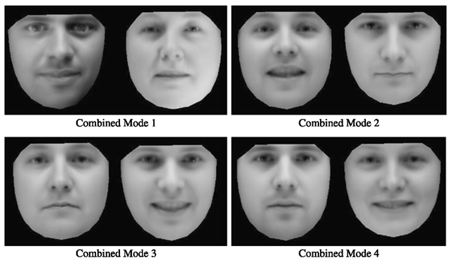
Fig. 5.5 Four modes of combined shape and texture model built from the same 400 face images as the texture-only model (Fig. 5.4). Combined parameters were varied by ±2 standard deviations from the mean

We therefore model these correlations by concatenating shape and texture parameter vectors into a single vector,

where Wi is a diagonal matrix of weights for each shape parameter, that accounts for the difference in units between the shape and texture models (see Sect. 5.1.3.1). We then apply a PCA on these combined vectors to give a model

where Pc are the eigenvectors and c is a vector of appearance parameters (with zero-mean by construction) that jointly controls both the shape and texture of the model. Note that the linear nature of the model allows us to express the shape and grey-levels directly as functions of c

An example image can then be synthesised for a given c by generating the shape-free, grey-level image from the vector g and warping it using the control points described by x to give images that combine variations due to identity, lighting, viewpoint and expression (Fig. 5.5).

Choosing Shape Parameter Weights

In the combined model, the elements of bs have units of distance whereas those of bg have units of intensity. As a result, applying unweighted PCA to the concatenated parameter vectors may incorrectly place greater emphasis on capturing variation in one more than the other. To address this problem, we first scale the shape parameters via the weighting matrix, Ws , so that the units of bs and bg are comparable.

A simple approach to choosing Ws is to set Ws = rI where r2 is the ratio of the total intensity variation to the total shape variation in the normalised frames. A more systematic approach is to measure the effect of varying bs on the sample g by displacing each element of bs from its optimum value for each training example and sampling the image given the displaced shape; the RMS change in g per unit change in shape parameter bs gives the weight ws to be applied to that parameter in (5.18). In practice, however, we have found that synthesis and search algorithms are relatively insensitive to the choice of Ws.

Separating Sources of Variability

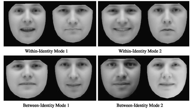
In many applications, some sources of appearance variation are more useful than others. In face recognition, for example, variations due to identity are essential whereas variations due to other sources (e.g., expression) are a nuisance whose effects we want to minimise. Since the combined appearance model mixes these two sources, each element of the parameter vector encodes both between- and within-identity variation. The sources can, however, be separated by splitting the subspace defined by Pc into two orthogonal subspaces,

where Pb and cb encode between-identity variation, and Pw and cw encode within-identity variation [24].

Computing the within-identity subspace is straightforward if we know the identity of the person in every training image—the columns of Pw are the eigenvectors of the covariance matrix computed using the deviation of each c from the mean appearance vector for the same identity. Varying cw then indirectly changes c and thus the appearance of the face but only in ways that a specific individual’s face can change, such as expression (Fig. 5.6, top).

The orthogonal subspace, Pb, that represents between-identity variation can then be computed by subtracting the within-identity variation, PwPTw c, and doing PCA over the resulting appearance parameter vectors. Alternatively, the between-class covariance matrix can be computed using the set of identity-specific means, though the mean is not guaranteed to be free of corruption by some non-neutral expression or head pose (Fig. 5.6, bottom). Iterative methods have also shown success in separating different sources of variability [16].

In contrast, tensor-based methods keep sources of variability separate at all times by building a multilinear model of texture variation [36, 60]. These methods, however, have strict requirements in terms of training data—namely, every combination of variation must be present in the training set (that is, every expression at every pose for every identity).

Fig. 5.6 (Top) Two within-identity modes of individual face variation; (bottom) two between-identity modes of variation between individuals. Some residual variation in expression is present due to not every mean face being completely neutral

Active Shape Models (ASMs)

Once we have built a statistical shape model from labelled training images, we need a method of matching the model to an unseen image of the face so that we can interpret the underlying properties of the image. One method, known as the Active Shape Model (ASM) [11], does this by alternating between locally searching for features to maximise a ‘goodness of fit’ measure and regularising the located shape to filter out spurious local matches caused by noisy data.

Goodness of Fit

Given a set of shape parameter values, b, and pose parameters, t, we can define the shape of the object in the image frame. If we also define a measure of how well given parameters explain the observed image data, we can find ‘better’ parameter values by searching in a local region around each feature point to find alternative feature locations that match the model more closely. In general, we can model appearance with a 2D patch centred at the feature location and search a 2D region of interest around the current estimate for better matches (see Sect. 5.2.5).

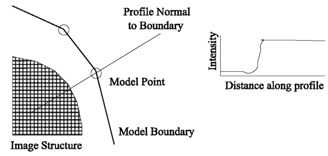
Fig. 5.7 At each model point, we sample along a profile normal to the boundary

In the specific case of the Active Shape Model [11], however, we reduce computational demands by looking along 1D linear profiles that pass through each model point and are normal to the model boundary (Fig. 5.7). If we assume that the model boundary corresponds to an edge, the strongest edge along the profile suggests a new location for the model point. Model points, however, are not always found on the strongest edge in the locality—they may instead be associated with a weaker secondary edge or some other image structure—and so instead we learn from the training set what to look for in the target image.

One popular method is to build a statistical model of the grey-level structure along the profile, normal to the boundary in the training set. Suppose for a given point we sample along a profile k pixels either side of the model point in the ;th training image. We then have 2k + 1 samples which can be put in a vector g;. To avoid the effects of a constant offset in the intensities (that is, differences in brightness), we sample the derivative along the profile rather than the absolute grey-level values. We similarly compensate for changes in contrast by dividing through by the sum of absolute element values such that

We repeat this for every training image to get a set of normalised samples, {g;}, whose distribution we can then model. If we assume that these profile samples have a multivariate Gaussian distribution, for example, we can build a statistical model of the grey-level profiles by computing their mean, g, and covariance, Sg. The quality of fit of a new sample, g^, to the model is then given by the Mahalanobis distance of the sample from the model mean,

and is related to the negative log of the probability that g^ is drawn from the learned distribution such that minimising f(gs) is equivalent to finding the maximum likelihood solution.

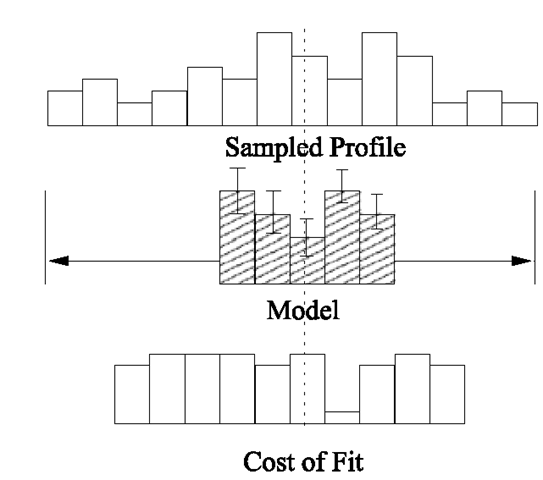
In practice, when performing a local search for a given feature point we first sample a profile of m > k pixels either side of the current estimate. We then test the quality of fit of the corresponding grey-level model to each of the 2 (m – k) + 1 possible positions along the sample and choose the one which gives the best match

Fig. 5.8 Search along sampled profile to find best fit of grey-level model

Algorithm 5.6: Active Shape Model (ASM) fitting

(as shown in Fig. 5.8) that is, the lowest value of f(gs). Repeating this for each feature point gives a new estimate for the shape of the face.