In Depth Tutorials and Information

Histogram Equalization (Image Processing) Part 1

In both the contrast stretching and window/level algorithms, monotonic and linear (and in the case of window/level, piece-wise linear) gray-level transform functions are applied to an image whose processed histogram yields an image of enhanced quality. In this section we consider a non-linear transform that takes into account the morphology of the input histogram. Consider the image shown in Figure 3-19a. One way to interpret the image’s discrete PDF (histogram) is to analyze its shape. Underutilized pixels correspond to valleys or shallow portions of the histogram, and if there were an algorithm that shifted pixel intensities such that the histogram was more evenly distributed, is it reasonable to assume that such a method would produce a better looking image? Figure 3-19c is the result of applying just such an operation, known as histogram equalization.

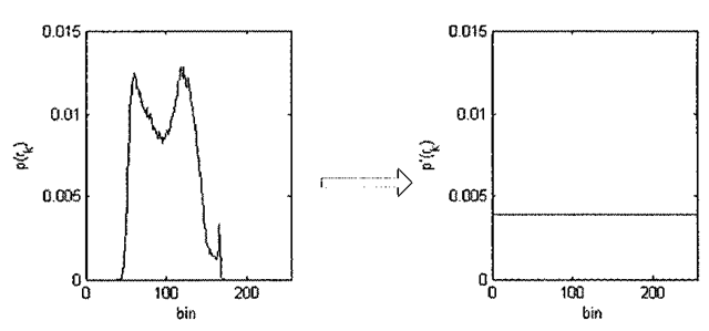
There are instances when histogram equalization can dramatically improve the appearance of an image, and this algorithm also forms a building block leading to a more general algorithm, histogram specification, that is used in image fusion applications. Histogram equalization alters the input histogram to produce an output whose histogram is uniform, where the various pixel intensities are equally distributed over the entire dynamic range. This situation is depicted in Figure 3-20. In the ideal continuous case, histogram equalization normalizes the pixel distribution such that the number of pixels in the image with pixel intensity p is MN/Q, where M is the number of image rows, N is the number of image columns, and Q is the number of gray-levels – in other words, a completely uniform probability density function whose value is constant. However, because digital image processing algorithms operate in the discrete domain, digitization effects come into play and prevent a purely uniform distribution, as evidenced by the shape of Figure 3-19d, where the equalized histogram is close to, but not exactly constant, over the interval 0-255.

So the goal of the histogram equalization algorithm is to find a gray-level transformation, of the now familiar form 5 = T(r), which makes the histogram p(rk) for A=0,1,…,Q-1 flat. The question now becomes how to find T(r)l For the purpose of this discussion, we normalize the allowable pixel range such that all pixel intensities are between 0 and 1, i.e. 0 < r < 1. We then assume the following two conditions:

1. T(r) is a monotonically increasing function that preserves the intensity ordering.

2. T(r) maps the range [0,1 ] to [0,1 ].

Figure 3-19. Histogram equalization, (a) Original image of birds at San Francisco Zoo. (b) Unprocessed histogram, (c) Histogram equalized birds image, (d) Equalized histogram, exhibiting an approximation to a uniform distribution across the range [0-255],

These two conditions are present for both the contrast stretching and window/level transforms, and if they hold, it is possible to define the inverse mapping s = T’x{r) because T is monotonic and single-valued. This inverse transform will in turn satisfy both (1) and (2).

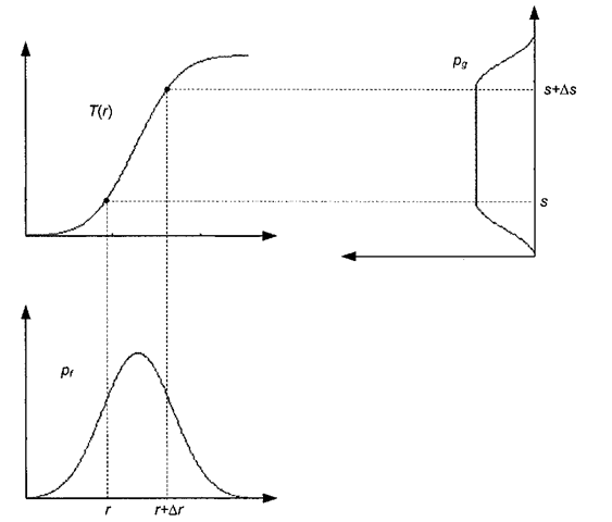
All of the pixels in the input image whose gray-levels lie within the range [r, r+Ar] will have their pixel intensities reassigned such that they lie within the range [.?, s+As], If pf (r) and pg (s) denote the PDFs of the input and output images, respectively, then the total number of input pixels with gray-level values lying between r and Ar is pj (r) Ar. Likewise, the number of output pixels with gray-level values lying between s and As is pg (s) As. Knowing what we do about T’l(s), the following condition must be true:

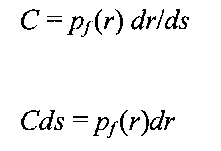
This equation basically states that for a given interval, the area underneath the two probability density functions p/(r) and pg (s) is the same (see Figure 3-21). If p/(r) is known, and T and T~l both satisfy condition 1, then it follows from probability theory that we can take the limit as both Ar and As go to zero and obtain

Since we desire a uniform distribution for the processed image pixels, the transform function T should adjust the gray-levels so that the output histogram is constant:

Plugging the above equation into the previous one yields:

Figure 3-20. Histogram equalization in the idealized case.

Figure 3-21. Histogram equalization in action. The transform function (top left) is such that the surface area under the curve Pf from r to r+Ar is the same as the surface area under the curve pg from 5 to .s+Aj. The plot of the output histogram pg is rotated by 90 degrees.

From the fundamental theorem of calculus, we can take the integral of both sides:

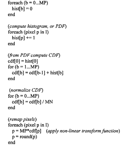
This integral is in fact the CDF of the distribution function pf(r) - so to construct the gray-scale transform function T(r) producing an output image whose histogram is approximately uniform, we first compute the CDF of the input image and then use it to remap the pixel intensities. As an example, consider Table 3-2 where we prepare to perform histogram equalization on a 10×10 3 bpp image. Such an image consists of 100 pixels, with pixel intensities ranging from 0-7. Starting with the discrete PDF (histogram) of the image (first three columns of Table 3-2), we next compute the CDF (cumulative histogram) of the image (last two columns of Table 3-2).

Table 3-2. Calculation of the CDF for histogram equalization._

Pixel	Histogram Count	PDF	Cumulative	CDF
Intensity		Pff)	Histogram
0	7	.07	7	.07
1	0	0	7	.07
2	13	.13	20	.2
3	15	.15	35	.35
4	6	.06	41	.41
5	15	.15	56	.56
6	32	.32	88	.88
7	12	.12	100	1.0
Total	100	1.0

In the next step, shown in Table 3-3, we use the CDF in conjunction with the maximum pixel intensity (in this case 7), to remap the pixel intensities. Note the properties of this mapping, namely that: