Euler Operations
Representation schemes based on using Euler operations to build objects are an attempt to have a boundary representation meet at least part of the validity issue head on. The idea is to permit only boundary representations that have a valid Euler characteristic. If we only allow operations that preserve the Euler characteristic or that change it in a well-defined way (such operations are called Euler operations), then we achieve this. Of course this is only a part of what is involved for an object not to be a nonsense object. Nevertheless we have at least preserved the combinatorial validity since the Euler characteristic is a basic invariant of combinatorial topology. As for metric validity, one still must do a careful analysis of face/face intersections. In any case, to say that a modeler is built on Euler operations means that it represents objects as a sequence of Euler operations.
Topologically, Euler operations are based on elementary collapses and expansions and/or cutting and pasting (see Sections 7.2.4 and 6.4 in [AgoM05], respectively). Figure 5.13 shows two elementary collapse and expansion examples. One says that the space Y consisting of the two segments on the right of Figure 5.13(a) is obtained from the solid triangle X on the left via an elementary collapse of the cell c from the edge e. Conversely, the space X is said to be obtained from Y via an elementary expansion. Figure 5.13(b) shows another elementary collapse and expansion, this time involving a three-dimensional cell ABCD and a face ABC. Figure 5.14 shows a cutting and pasting example. Specifically, we show how to cut the torus to get a rectangle and how, looking at it backward, we can get the torus from the rectangle by pasting appropriate edges together.
Figure 5.13. Elementary collapses/expansions.
Figure 5.14. Cutting and pasting.
Elementary collapses or expansions do not change the Euler characteristic of a space. On the other hand, cutting and pasting operations usually do change the Euler characteristic. It turns out that these four operations do an excellent job to completely describe and define surfaces. (In higher dimensions things get more complicated.) Every surface, and hence solid in 3-space, can be obtained from a point by a sequence of elementary expansions, cuts, and pastes. Modelers based on Euler operations use a boundary representation for solids and simply define procedures that mimic the collapses, expansions, cutting, and pasting operations just described by modifying the cell structure of this boundary representation in a well-defined way.
Definition. The Euler operation representation of polyhedra is defined by the collection of pairs![]() where X is a polyhedra and
where X is a polyhedra and is a sequence of Euler operations that produces
 starting with the empty set.
Euler operations were first introduced by Baumgart in his thesis and then used in his computer vision program GEOMED ([Baum75]). Braid, Hillyard, and Stroud ([BrHS80]) showed that only five operators are needed to describe the boundary surfaces of three-dimensional solids. Such a surface satisfies the Euler equation
where
They used a set of these Euler operations in their BUILD modeling system. Although one can make other choices for the five primitive operators, it seems that the boundary representation part of modelers built on Euler operations tend to use either
Figure 5.15. Building a tetrahedron with Euler operations.
Baumgart’s winged edge representation (see Section 5.8.1) or some variant of it, so that this is what these operators modify.
Historically, Euler operators were given cryptic mnemonic names consisting of letters. A few of these are shown below along with their meanings:
Using that notation, three typical operators were:
Figure 5.15 shows how one could create a solid tetrahedron using these operators. The operators create the appropriate new data structure consisting of vertices, edges, faces, and solids and merge it into the current data structure. Along with each Euler operator that creates vertices, edges, or faces, there are operators that delete or kill them. This enables one to easily undo operations, a very desirable feature for a modeler.
To summarize, modelers based on Euler operations are really "ordinary" b-rep modelers except that the objects and boundary representations that can be built are constrained by the particular Euler operators that were chosen, so that they at least have combinatorial validity. The Euler operators are flexible enough though so that the modelers share all the advantages (and some of the disadvantages) that one gets with a boundary representation.
We need to leave the reader, at least those who might be interested in modeling objects in higher dimensions than three, with one word of caution however. The result about five operators sufficing to construct objects raises some subtle issues. It applies only to the two-dimensional boundaries of solids and not to cell structures of solids. The fact is that not all n-cells, n > 2, are shellable (another term for collapsible)] For a proof see [BurM71]. To put it another way, the higher-dimensional analogs of the Euler operators are not adequate for creating all cell decompositions of higher-dimen-sional objects.
Sweep Representations and Generative Modeling
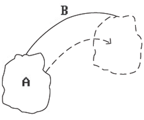
Sweep representations correspond naturally to the way many mechanical parts are manufactured. The basic idea of this scheme is to "sweep" one set A along another B. See Figure 5.16. There are several different types of sweeps.
|
Translational sweeps: |
These are common in sheet metal systems. See Figure 5.17(a). |
|
Rotational sweeps: |
These are used in the context of turned or lathed parts. See Figure 5.17(b). |
|
Solid sweeps: |
These are used with milling machines. See Figure 5.17(c). |
|
General sweeps: |
Not much is known in this case because sweeping even nice sets along simple paths can produce nonsolids. See Figure 5.18. It is difficult to guarantee that swept objects will be solids. |
Figure 5.16. Sweeping an object along a curve.
Figure 5.17. Sweep operations.
Figure 5.18. Problem with sweeps.
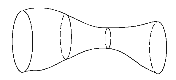
Figure 5.19. Generalized cylinder.
Sweeps sometimes become inputs to other representations. For example, in CADD (a program developed by McDonnell Douglas) one can translate certain sweep representations, such as translational and rotational ones, into boundary representations.
Related to sweeps is the multiple sweeping operation using quaternions described in [HarA02]. There are also the generalized cylinders of Binford ([Binf71]). See Figure 5.19. Here the "sweeping" is parameterized. We shall now discuss a representation scheme developed by J. Snyder at Caltech that is more general yet.
Definition. A generative model is a shape generated by a continuous transformation of a shape called the generator.
Arbitrary transformations of the generator are allowed. There is no restriction as to the dimension of the model. The general form of a parameterization S(u,v) for a generative model which is a surface is
where is a curve in
 is an arbitrary function. One
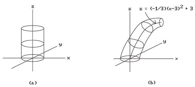
of the simplest examples of this is where one sweeps a circle along a straight line to get a cylinder. Specifically, let
be the standard parameterization of the unit circle. Define f by
Figure 5.20. Generative models.
See Figure 5.20(a). A more interesting example is shown in Figure 5.20(b) where we use
and Rv is the rotation about the y-axis in R3 through an angle of![]() This corresponds to sweeping the unit circle along the parabola
This corresponds to sweeping the unit circle along the parabola
in the xz-plane. The circle gets rotated and scaled by a factor of 1 – v/6 as we move it.
The parameterization S(u,v) in equation (5.3) can be thought of as defining a one-parameter family of curves![]() defined by
defined by![]() As the examples in Figure 5.20 suggest, this family of curves can correspond to a fixed curve being operated on by quite general transformations as it is swept along arbitrary curves. This is, in fact, one reason for creating the generative model representation, namely, that it allows powerful operators for modifying objects.
As the examples in Figure 5.20 suggest, this family of curves can correspond to a fixed curve being operated on by quite general transformations as it is swept along arbitrary curves. This is, in fact, one reason for creating the generative model representation, namely, that it allows powerful operators for modifying objects.
More generally, generative models of arbitrary dimension have parameterization S(u,v) of the form
where![]() This is thought of as a (k + s)-dimensional model obtained by sweeping a k-dimensional object along an s-dimensional path. For example, this allows us to define solids as generative models. A common representation is to represent a solid as sweeping an area along a curve.
This is thought of as a (k + s)-dimensional model obtained by sweeping a k-dimensional object along an s-dimensional path. For example, this allows us to define solids as generative models. A common representation is to represent a solid as sweeping an area along a curve.
Definition. The generative modeling representation consists of pairs (X,F), where F is a parameterization of the generative model X of the form shown in equation (5.4).
The driving force behind GENMOD was correcting some perceived deficiencies in the geometric modeling systems of that time and some key defining points listed by [Snyd92] for the generative modeling approach as implemented in GENMOD are:
(1) The representation is a generalization of the sweep representation.
(2) Shapes are specified procedurally.
(3) Specifying a shape involves combining lower-dimensional shapes into higherdimensional ones.
(4) An interactive shape description language allows low- and high-level operators on parametric functions.
(5) It is closed, that is, the outputs to operations can be inputs to operations (like CSG).
(6) It allows parameterized shapes whose parameters a user can change.
(7) It supports powerful high-level operators and functions, such as reparameterizing a curve by arc length, computing the volume of a shape enclosed by surface patches, and computing distances between shapes.
These operations are closed and free of approximation error.
(8) It supports deformation operators, CSG, and implicitly defined shapes.
(9) One has the ability to control the error in the representation.
A large variety of symbolic operators on the parameterizations and their coordinates help the user define generative models, such as vector and matrix operations, differentiation (partial derivatives), integration, concatenation, and constraint operators. Since parameterizations can be thought of as vector fields, another useful operator is one that solves ordinary differential equations. GENMOD had a language in which a user could define models using the various operators.
Now, models will have to be displayed. By converting to polygonal meshes and ad hoc error control, the interactive rendering of generative models becomes feasible. One can specify the subdivisions in two ways: uniform in domain or adaptive sampling. More realistic images can be obtained at the expense of speed.
For accuracy, GENMOD used interval analysis. Interval analysis is an attempt to make numeric computations on a computer more robust and has its advantages and disadvantages. Snyder argued for its use in geometric modeling and described various applications to computing nonintersecting boundaries of offset curves and surfaces, approximating implicitly defined curves and surfaces, and trimmed surfaces and CSG operations on them.
In summary, three more advantages used by Snyder to justify the generative modeling approach are:
(1) The representation handles all dimensions, is high-level, and extensible.
(2) Using a high-level interpreted language, the mathematically knowledgeable user can easily build a library of useful shapes.
(3) An adequate number of robust tools for rendering and manipulating generative models exist.


