Wavelet-Based Filtering Part 1 (Biomedical Image Analysis)

We discussed the decomposition of a signal (or image) into a lowpass- and highpass-filtered component. Wavelet-based filters can be envisioned as algorithms where wavelet decomposition takes place, followed by an attenuation of either the lowpass-filtered component or the highpass-filtered component. An inverse wavelet transform then restores the filtered image. The underlying principle can be seen in Figure 4.8. The H/H area of the decomposed image contains mostly noise, whereas the L/L area contains most of the lower-detail image information. A smoothing or noise-reducing filter would attenuate the wavelet coefficients at higher scales (i.e., wavelet coefficients containing image detail). Sharpening filters or background removal filters would attenuate the lowpass-filtered wavelet coefficients at a high level of decomposition, in analogy to lowpass filtering in the Fourier domain. Although some work has been done in detrending signals by using the wavelet transform, wavelet-based background removal has not entered the mainstream of image processing. In fact, the most widely used wavelet-based filtering technique is the noise-reducing filter analogous to the Fourier-domain lowpass filter. Contrary to the Fourier lowpass filter, however, wavelet-based noise-reduction filters do not blur the image edges significantly. The removal of noise from images using wavelet techniques is far superior to that using Fourier techniques, and the term denoising has become common in conjunction with wavelet filtering techniques to indicate almost complete noise removal, as opposed to noise attenuation or noise reduction performed using Fourier techniques with lowpass filters or convolution filters.

Algorithm 4.4 Discrete wavelet transform. Pseudocode to perform a one-dimensional wavelet transform on the input data array xdata[] with a total length of N elements. The output vector is also in xdata[]. With the variable maxlevel, the number of decomposition steps can be restricted.

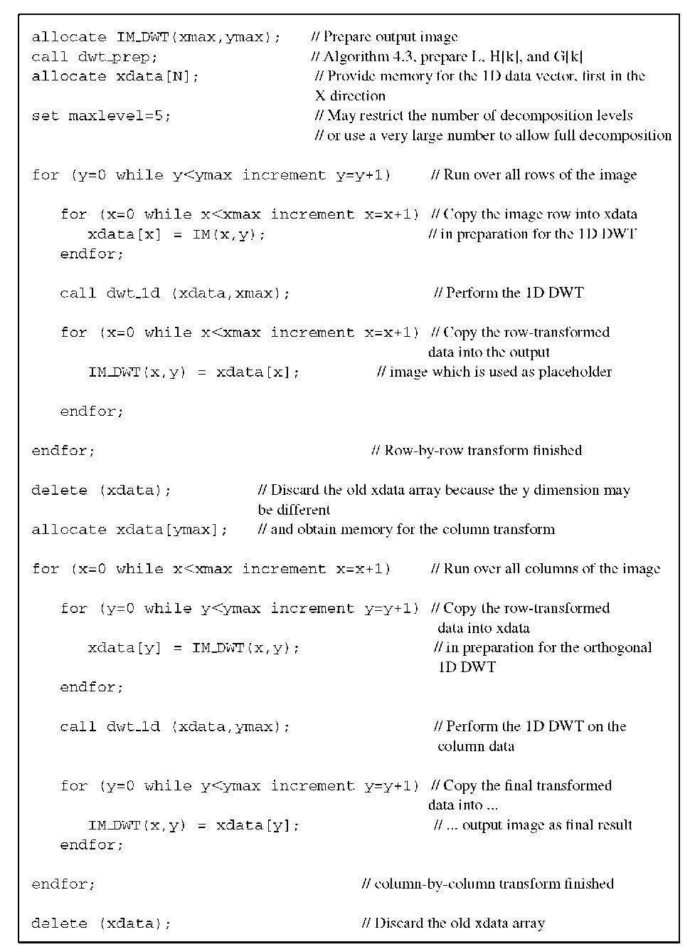
Algorithm 4.5 Discrete wavelet transform in two dimensions. Pseudocode to perform a two-dimensional wavelet transform on the input image IM(x,y). It is assumed that the image dimensions xmax and ymax are powers of 2. The data are stored in the output image IM_DWT(x,y) with the same dimensions as IM(x,y) and which, upon exit, holds the discrete wavelet transform of IM. 

Wavelet-Based Denoising

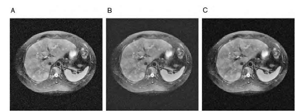
Denoising filters involve more complex operations than simply eliminating the wavelet coefficients in the H/H area before reconstruction. The effect is demonstrated in Figure 4.9, where high-frequency areas L/H, H/L, and H/H of the first-level decomposition were set to zero before reconstruction. The noise is hardly attenuated, but resembles more closely the output of a Gaussian convolution filter.

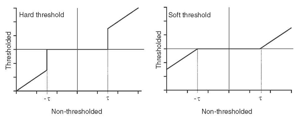
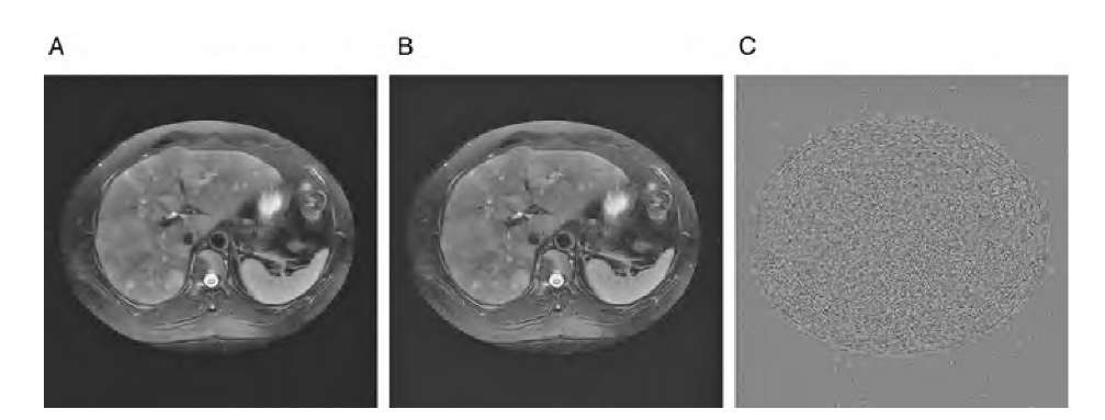
A robust method of wavelet-based denoising was proposed by Donoho.12,13 Here, the wavelet coefficients are subjected to a hard or soft threshold as shown in Figure 4.10. This operation is termed wavelet coefficient shrinking. The result of applying a wavelet shrinking filter to the image in Figure 4.9A is shown in Figure 4.11. It can be seen that noise suppression is considerably stronger than in Figure 4.9B, whereas edge blurring, associated with a Gaussian blurring operation (Figure 4.9C), is less pronounced. As a generalization, hard thresholding leads to a smaller mean-squared error between the ideal noise-free image and the noisy image, whereas soft thresholding has a lower tendency to cause spurious oscillations in the reconstructed image. These oscillations may be related to Gibbs phenomena7 and can be suppressed by the following averaging technique: Multiple denoising operations are performed where the original image is cyclically shifted by one or multiple pixels for each wavelet denoising operation. After reconstruction, the image is shifted back in the same manner. Since those oscillations occur where image discontinuities and wavelet discontinuities coincide, the average of the images filtered by the shift-denoise-unshift operation will exhibit attenuated oscillations.

Donoho and Johnstone propose t = V2logn as a universal threshold,13 but the optimum global threshold t depends on the noise component, more specifically the noise standard deviation ct. If ct is known, the following equation provides a better threshold value:

FIGURE 4.9 A first approach at attenuating noise in an image using the wavelet transform. The original image in Figure 4.8, a MRI slice with artificially added Gaussian noise (A), was decomposed as shown in Figure 4.8B, and the L/H, H/L, and H/H regions set to zero before reconstruction (B). The resulting image shows a considerable noise component, but on a coarser scale, very similar to the result of Gaussian blurring (C).

FIGURE 4.10 Thresholding schemes for wavelet coefficient shrinking. With a hard threshold, every wavelet coefficient 7 is either clamped to zero if 7 falls below the threshold (hard thresholding) or all coefficients are set to zero ifand all coefficients withare reduced by the threshold t (soft thresholding).

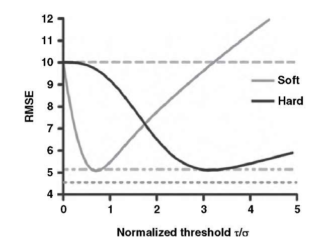
Here n is the total number of wavelet coefficients, ct the standard deviation of the noise component, and Y an empirical constant that determines filter strength. The effect of the threshold on the filtered image quality can be seen in Figure 4.12, which shows the root-mean-squared error (RMSE) of the wavelet filter output image and the original noise-free image. It can be seen that the selection of a suitable threshold value has a major influence on the filtered image. A low threshold value reduces the efficacy of the filter, and a significant noise component is left in the image. High threshold values lead to the removal of image detail and cause block artifacts in the reconstruction. For comparison, the RMSE values of a Gaussian blurring filter and a median filter are shown. Although both median filter and Gaussian blurring yield good RMSE values, the perceived quality of the wavelet-filtered image is superior because it retains its edge information. The choice of wavelet function for decomposition and reconstruction also has an influence on the filter efficacy. The example in Figure 4.12 was created by using the Daubechies-4 wavelet. With the Haar wavelet and soft thresholding, the minimum RMSE is 5.44, compared to 5.1 when using the Daubechies-4 wavelet. An even smoother wavelet, theDaubechies-12 wavelet, reduces the RMSE to 4.88, whereas no further reduction is seen with the Daubechies-20 wavelet. The influence of the wavelet choice on the reconstructed image can be seen in Figure 4.13. With the Haar wavelet, the reconstruction appears to have square patches, which are particularly visible in the liver area. With both Daubechies wavelets, the tissue seems to blur into the background (stronger with the Daubechies-20 wavelet).

FIGURE 4.11 Denoising of the image in Figure 4.9A using the Donoho algorithm. Soft thresholding (A) leaves some visible noise, especially in the background region. Hard thresholding, although having approximately the same root-mean-squared error (B), shows less residual noise but some oscillation artifacts. These oscillations are emphasized in image C, which is the difference between filtered image B and the original, noise-free image. Image C has been slightly contrast-enhanced for better visualization.

FIGURE 4.12 Root-mean-squared error (RMSE) between the denoised image and the original, noise-free image as a function of the threshold. The dashed lines indicate, from top to bottom, the RMSE of the unfiltered image, the RMSE of the image filtered with a median filter, and the image filtered by Gaussian blurring.

Many wavelet denoising approaches are based on the wavelet shrinkage filter developed by Donoho and Johnstone.12,13 The statistical modeling of the wavelet coefficients is an important step toward automated determination of the optimum shrinkage threshold.27 Donoho and Johnstone13 suggested using the median absolute wavelet coefficient, divided by 0.6745, as an estimator for the noise variance:

FIGURE 4.13 Influence of the wavelet choice on the reconstructed, denoised image. In all cases, a gamma contrast-enhancement function has been applied to make the background texture more visible. Image A was reconstructed using the Haar wavelet, for image B the Daubechies-12 wavelet was used, and for image C the Daubechies-20 wavelet was used.

This estimate can be used for ct in Equation (4.20). This approximation is valid only if the noise component is zero-mean, Gaussian, uncorrelated, additive noise. In other words, each wavelet coefficient 7 (k) is a superposition of the "clean" wavelet coefficient 7 0 (k) from the idealized, noise-free image and a contribution e(k) from additive Gaussian white noise, that is,

Another proposed model23 that leads to a spatially adaptive filter also assumes that the wavelet coefficients contain an additive zero-mean, Gaussian-distributed random component but with a high local correlation and known global standard deviation ctn . In this case, an estimate for 7 0 (k) can be given that uses a local minimum mean-squared-error method:

The local variance CT2(k) can be estimated by using

under the assumption that the wavelet coefficients are distributed with an exponential probability function:

In Equation (4.23), the local neighborhood around pixelsquare neighborhood) and contains N elements. The exponent \ can be determined by computing the histogram of local variances for the wavelet coefficients and by fitting the function in Equation (4.24) to the histogram. In the actual denoising process, each highpass coefficient 7 (k) is replaced by the estimated noise-free coefficient 70(k), and the resulting wavelet coefficient image is subjected to the inverse wavelet transform.

Yet another technique used to find an optimum threshold for wavelet shrinkage is the generalized cross-validation (GCV) technique.17 Generalized cross-validation entails finding a threshold t so that the GCV estimator, G(t ), is minimized in the equation

where the 7l (i) are the original highpass wavelet coefficients at decomposition level l, the 7l (i) are the wavelet coefficents after application of threshold t , Nl is the total number of wavelet coefficients at decomposition level l, and Tl is the number of wavelet coefficients that have been set to zero as a consequence of the thresholding process. It is important that hard thresholding be used for the computation of the 7l(i) and G(t ). Once the value for t that minimizes G(t ) has been found, the 7l(i) are used to reconstruct the image through the inverse wavelet transform. The estimator G(t ) is computed for, and applied to, each decomposition level independently.

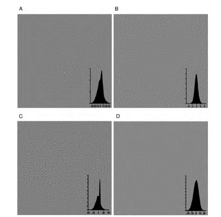
The denoising performance of the three unsupervised threshold functions described above can be seen in Figure 4.14. The example is again based on the noisy MR slice in Figure 4.9A and a three-level decomposition using the Daubechies-12 wavelet. From Figure 4.14 it can be seen that the universal threshold underestimates the noise component in strongly noise-affected images. Multiplying the universal threshold with the estimated standard deviation, obtained through Equation (4.21), gives a very high threshold that is optimal with respect to RMSE and coincides with the threshold in Figure 4.12, where the hard-threshold minimum RMSE was found. The histogram shows a deviation from the Gaussian shape and therefore indicates that image information was removed in the filtering process. Also, the reconstruction shows block artifacts (compare to Figure 4.11B). The filter used for Figure 4.14D differs from Figure 4.14B and C insofar as individual threshold values were determined for each decomposition level. The optimization of the GCV [Equation (4.25)] is performed for each decomposition level. Applying an optimized threshold for each decomposition level provides noise removal close to the actual added noise component with no visible image structures removed.

The GCV algorithm is not difficult to implement. Although more efficient minimum-search methods exist, a simple brute-force approach provides a suitable starting point. A suggested implementation of GCV-based denoising is presented in Algorithm 4.6. This algorithm performs an in-place wavelet shrinkage on the wavelet-transformed image W(x,y), and uses the function thresh(coeff,t) to perform hard thresholding on a coefficient coeff with threshold t. This function compares the absolute of coeff with t and returns the value of coeff if |coeff|>t and zero otherwise. Also, a reasonable upper bound for the threshold, uthresh, needs to be specified. In the simplest case, this variable may be set to the largest wavelet coefficient in the input image.

FIGURE 4.14 Comparison of the denoising efficacy of three automated threshold-finding algorithms with conventional Gaussian blurring. Shown is the noise component removed from Figure 4.9A, that is, difference between image 4.9A and the filtered image. The insets show the gray-value histograms of the various images. In image A, conventional Gaussian blurring was applied. The difference image clearly shows the noise removed in most areas, but it also contains image information: namely, the edges that get blurred in the smoothing process. Image B was produced using Donoho’s universal threshold, image C used a threshold based on an estimate of a through Equations (4.20) and (4.21), and image D was produced using general cross-validation, Equation (4.25). In the latter case, the noise component is almost identical to the artificially added noise, and no structural elements can be seen in the difference image.