Fourier-Based Filtering (Biomedical Image Analysis)

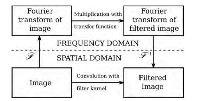
In Section 3.1, the possibility of using the Fourier transform to remove periodic components from images was introduced briefly. However, frequency-domain filtering is far more comprehensive. The foundation of frequency-domain filtering is the convolution theorem, which stipulates that a convolution in the spatial domain corresponds to a multiplication in the Fourier domain. Computational effort of a convolution increases with K2N2 on N x N images and K x K kernels. With the fast Fourier transform, computational expense is reduced to 2 N log2 N and N x N additional multiplications. On large images and large convolution kernels, Fourier filtering is considerably faster. Furthermore, due to the defined spatial frequencies, the action of the Fourier-domain filter can be dramatically better adjusted than that of convolution filters (which often are merely approximations of filter functions in a small neighborhood, such as a 3 x 3 kernel). A Fourier-domain filtering process includes three steps: computation of the Fourier transform of the image; multiplication with the filter function and computation of the inverse Fourier transform (Figure 3.8). A fourth and optional step, windowing, is discussed later in the topic.

Two of the most commonly used filter types are lowpass filters (where the higher frequencies are attenuated) and highpass filters (where the low-frequency components are attenuated). Lowpass filters have noise-attenuating properties and blur the image. Lowpass filtering is associated with a loss of detail and with softening of sharp transitions. Highpass filtering enhances edges and may be used to remove inhomogeneous background components. Highpass filters also tend to increase the noise component. Bandpass filters and notch filters are used less frequently in image processing. A bandpass filter emphasizes specific periodic components, whereas a notch filter suppresses periodic components. The band of frequencies that are not attenuated is called the passband, and the band of frequencies that are attenuated is called the stopband. The frequency at which the transition between passband and stopband takes place is the cutoff frequency.

FIGURE 3.8 Filtering in the frequency domain. Instead of filtering the image in the spatial domain by convolving the image with the filter kernel, the image can be transformed into frequency space by using the FFT (indicated by the symbol F). The Fourier transform of the image is then multiplied by the filter function (also called the transfer function, i.e., the Fourier transform of the convolution kernel), and the resulting frequency-space filtered image is subjected to the inverse Fourier transform (F-1). Although this "detour" into the frequency domain may appear to be additional effort, the overall computational expense is dramatically less than for a convolution with large kernel sizes.

Filters are usually designed to act equally on all spatial frequencies, making them rotationally symmetrical [see Equation (3.10)]. Furthermore, filter functions are designed to achieve a smooth transition between frequency components that are allowed to pass and those that are blocked. Steep transitions cause an artifact known as ringing. For this reason, a filter function such as a lowpass filter with a frequency response H(w),

with the cutoff frequency w0 is not advantageous and not normally used. 3.2.1. Lowpass Filters

Lowpass filters are used primarily for noise reduction. They remove image detail and blur the image. Lowpass filters are often applied in preparation for segmentation to reduce the influence of noise. In the spatial domain, blurring is often performed by a convolution with an approximated Gaussian kernel. Interestingly, the Fourier transform of a Gaussian function is again a Gaussian function. Therefore, a popular lowpass filter is a filter with Gaussian-shaped frequency response

whereis the spatial frequency, A is the overall gain, and ct is the width (steepness).

where the function clamp(x) is 0 for x < 0 and x for x > 0. With the help of the clamp function, the passband frequencies are extended such that all frequency components below w0, the cutoff frequency, remain unchanged.

Another frequently used lowpass filter function is the Butterworth filter. Its filter function has the steepest possible transition between passband and stopband without passband ripples (ringing). Its frequency response is

where A is the overall gain, w0 the cutoff frequency, C an asymmetry factor, and n the order.

Selection of the filter and the filter parameters is often empirical. Examples of the action of the filters are shown in Figure 3.9. Whereas similarly adjusted lowpass filters with Gaussian and Butterworth characteristics (Figure 3.9B and C) are visually similar, the edges are blurred less strongly with the Butterworth filter. The effect of a steep transition (ripples or ringing, seen as periodical oscillations near edges) is demonstrated in Figure 3.9D where a Butterworth filter of order n = 25 was used.

Highpass Filters

An alternative implementation uses

In general, highpass filters Hhp(w) can be obtained from lowpass filters HLP(w) through

provided that the passband gain is normalized to unity. In the example of the But-terworth lowpass filter [Equation (3.18)] application of Equation (3.19) leads to the complementary Butterworth highpass filter,

The choice of a relatively steep filter with a low cutoff frequency provides a filter that partly removes an inhomogeneous background (an image component with a very low frequency), while a higher cutoff frequency leads to a distinctly edge-enhancing filter, similar to convolution-based edge detectors. Specifically for the removal of an inhomogeneous background, the filter is more suitable. In this filter, s is the steepness, w0 the cutoff frequency, and A an offset that can be used to adjust the strength of the filter. After application of the filter in Equation (3.21), the value range needs to be normalized if A = 0. Examples of the application of these filters are shown in Figure 3.10.

FIGURE 3.9 Effect of Fourier-domain lowpass filters. The original image is a high-contrast version of the Shepp-Logan head phantom with additive Gaussian noise and a gradual background gradient (A). A Gaussian lowpass filter with ct = 30 pixel-1 [B; left half: Equation (3.16), right half: Equation (3.17) with w0 = 20 pixel-1] reduces noise but also causes some degradation of the edges (blurring). A second-order Butterworth filter [Equation (3.18), w0 = 66 pixel-1, C = 1] produces a similar effect (C). If the transition from the passband to the stopband is very steep, for example, by using a high-order Butterworth filter (D, same parameters as C except that n = 25), edges are accompanied by spatial oscillations ("ringing").

Very frequently, the filter in Equation (3.21) is applied in a multiplicative manner. In this case, the filter is known as a homomorphic filter. The underlying assumption is inhomogeneous illumination, where the image values I(x,y) are the product of nonuniform illumination intensity I0(x,y) and the reflectance (or transmittance) of the imaged object, O(x,y). In logarithmic form, the product becomes a sum, log I(x,y) = log I0(x,y) + log O(x,y). The illumination intensity function I0(x,y) is assumed to have only low-frequency components. When the log-transformed data log I (x,y) are filtered with the filter in Equation (3.21), the low-frequency additive component log I0(x,y) is strongly attenuated, and only the object component remains. By raising the filtered log-transformed image to the power of 10, the original image is restored with the multiplicative background inhomogeneity removed.

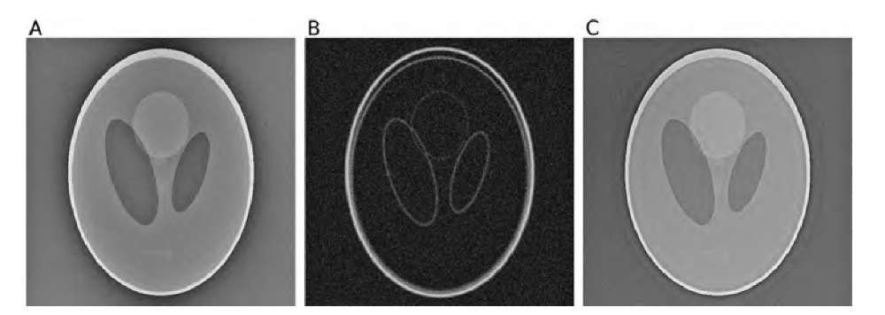
FIGURE 3.10 Highpass filtering of the phantom in Figure 3.9A. A Butterworth filter with low cutoff frequency (w0 = 2 pixel-1, C = 1, n = 1, A = 1) partly removes the background inhomogeneity, but it also introduces a new region of reduced intensity around the edge (A). With a higher cutoff frequency (w0 = 25 pixel-1), the filter assumes a strong edge-enhancing characteristic, particularly when the absolute values are taken (B). The filter in Equation (3.21) (w0 = 20, A = 2, s = 0.5) effectively removes the background inhomogeneity (C) while exhibiting less of the reduced-intensity area around the phantom than does the Butterworth highpass in part A.

Wiener Filters

Frequency-domain filters play an important role in image restoration. Any imaging device has a certain point-spread function (PSF), that is, the image function of an idealized point source. For an optical system, the PSF could be measured by acquiring the image of a back-illuminated pinhole. For a CT system, the PSF could be determined by imaging a thin axial wire. Most frequently, the PSF has a Gaussian shape. If the point-spread function g(x,y) of an imaging device is known, any image I(x,y) obtained by this device can be seen as the convolution of an idealized image I’(x,y) with g(x,y). Let G(u,v) = F{g(x,y)} be the Fourier transform of g(x,y); then degradation by the PSF can be described in the frequency domain by

The idealized but inaccessible image I’(x,y) can therefore be restored by deconvolu-tion, that is, division by the PSF in the frequency domain, described by

The problem with this approach is that the point-spread function G(u,v) has a low-pass character, which means that the values of G(u,v) become very small for large u and v. Since the measured image data I(x,y) usually contain noise, the Fourier transform of I(x,y) also contains noise. This noise component is broadly distributed and a considerable amount of noise exists in the Fourier transform of the image for large u and v, where the division by small values of G(u,v) causes a massive noise amplification. Therefore, if an image is degraded by a lowpass point-spread function and additive noise, it is not possible to reconstruct the undegraded image. However, a filter function can be designed that provides an optimum estimate that minimizes the squared distance between I and I’. This best-estimate filter is called a Wiener filter. Often, the noise component can be measured or estimated, for example, by analyzing a flat region of the image. A common model is additive noise, where each pixel contains a noise component e(x,y) with zero mean and a standard deviation of ct. It can be shown that the best-estimate filter is the function W(u,v):

where G*(u,v) is the conjugate complex of the frequency-domain PSF, N(u,v) is the estimated Fourier spectrum of the noise, and I(u,v) is the Fourier spectrum of the original image and approximately similar to the Fourier spectrum of the degraded image, provided that the degradation is minor. To obtain the best-estimate approximation of the ideal image, the degraded image needs to be multiplied in the Fourier domain with W(u,v), and Wiener filtering becomes the process

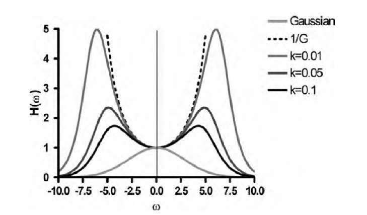
In this case, k can be adjusted manually to provide an acceptable approximation of the restored image. The main effect of the real-valued scalar k is to prevent the filter function 1/G(u,v) from assuming very large values for large u and v and thus amplifying the noise component. The effect of the Wiener filter and the choice of k are illustrated in Figure 3.11.

Cross-Correlation and Autocorrelation

Cross-correlation is a method for template matching. A template, g(x,y), is slid over the image I(x,y) and overlapping pixels are summed up. This is, in fact, equivalent to a convolution operation

Sometimes the Wiener filter is implemented with an adjustable parameter k:

FIGURE 3.11 Frequency response of a Wiener filter as defined in Equation (3.26). Assume that the degradation function G(w) is a Gaussian function (light gray line); then its reciprocal (dashed line) assumes very large values at moderate to high spatial frequencies. Multiplication of a degraded image by the reciprocal would strongly amplify noise. Instead, a Wiener filter can be used to attenuate very high frequencies. The frequency response of the filter in Equation (3.26) is shown for three different choices of k.

The template g(x,y) and similar shapes can be found at peak locations of C(x,y). By using the convolution theorem, the convolution in Equation (3.27) can be written as a multiplication in the frequency domain:

where G*(u,v) is the conjugate complex of the Fourier transform of g(x,y). The autocorrelation is the cross-correlation of the image with itself, and Equation (3.28) applies in the same manner.

Filter Implementation and Windowing

For the implementation of symmetrical lowpass and highpass filters, a filter function can be provided that returns H(w) for any given w. To filter an image with this filter function, the image needs to be subjected to a FFT, and the FFT image data need to be rearranged so that the zero-frequency element F(0,0) is in the center. In a loop over all pixels (u,v) of the FFT image, the frequency response is obtained by computing w as the Euclidean distance of (u,v) from the center and calling the filter function to obtain H for this frequency. Both the real and imaginary parts of the FFT values are then multiplied by H. Once all pixels are processed, the resulting filtered FFT image is subjected to the inverse Fourier transform. Since the result of the inverse FFT is usually complex-valued, the imaginary component can be discarded (it should contain values very close to zero, anyway) and the resulting spatial-domain real-valued pixel values rounded to fit the original image depth.

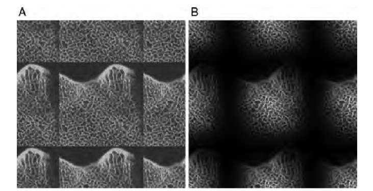
FIGURE 3.12 Discontinuities at the edges of images that are assumed to be periodic. The example shows a magnified section of an x-ray image of bovine bone. The Fourier transform assumes that images are 2^-periodic, that is, infinitely tiled, as illustrated in part A. This creates discontinuities at the image edges with associated high-frequency components. By multiplying the image by a window function, the image values at the edges are attenuated and a forced continuity at the edges is created (B).

An important consideration for the implementation of Fourier-domain filters, even for the estimation of spectral components, is the assumed periodicity of the image. In Section 3.1 the Fourier transform was introduced under the assumption that any signal is 2^–periodic, and any image consequently is 2^–periodic in both directions. It was also explained that edges create high-frequency components. Discontinuities between image values at the left and right border and at the upper and lower border also count as discontinuities, as can be seen in Figure 3.12. These discontinuities create additional high-frequency components in the Fourier transform. To prevent these high-frequency components, it is recommended that the image be multiplied by a window function in the spatial domain, a process called apodization. The window function attenuates image values toward the edges and therefore reduces the discontinuity (Figure 3.12B). After filtering and inverse Fourier transform, the original image values are restored by dividing the filtered image by the window function.

A window function has its own frequency response. For this reason, smooth window functions are preferred that contribute only minimally to the frequency spectrum. One example window function is

where M and N are the image dimensions in the x and y directions, respectively. With the choice of a = 0.5 and b = 0.5, this window is known as the Ham window, and with a = 0.54 and b = 0.46, the window function becomes the Hamming window. The Hamming window is one specific form of raised cosine window where the window values do not drop to zero at the edges. This is important for recovery of the image values after the inverse Fourier transform, because edge pixels where w(x,y) drops to zero cannot be recovered by dividing by w(x,y). Other windows of linear (Bartlett window), parabolic (Welch window), or Gaussian shape exist. In the practical application the exact choice of the window function will not have a measurable impact on the filtered image as long as the window function approaches zero smoothly toward the edges of the image.

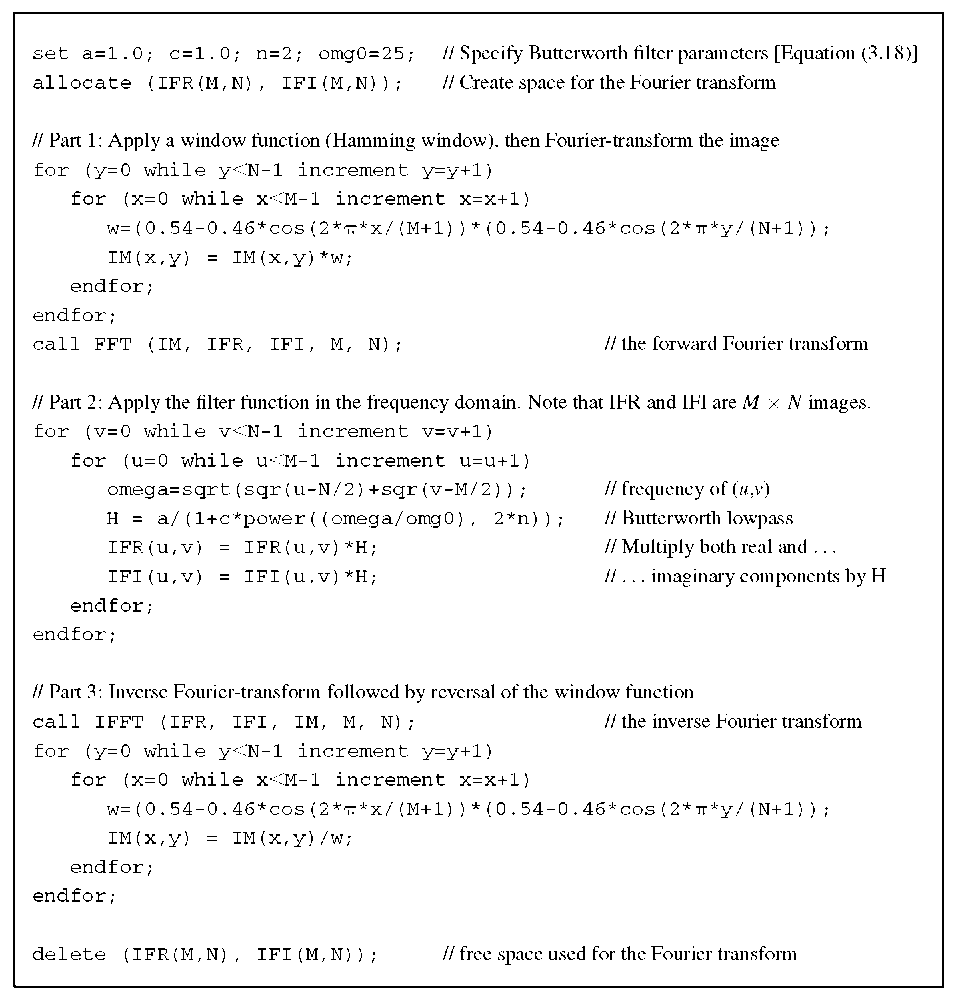
The summary of these steps is presented in Algorithm 3.2. The algorithm relies on two external functions, FFT and IFFT, which perform the forward and inverse Fourier transforms, respectively, in the image IM and its real and imaginary parts of the Fourier transform, IFR and IFI.

Algorithm 3.2 Fourier-based filtering using the example of a Butterworth lowpass filter. This algorithm relies on external functions to perform the Fourier transform. FFT transforms image IM and generates the real part IFR and the imaginary part IFI of the Fourier transform. The inverse transform function IFFT takes IFR and IFI and returns IM. This algorithm demonstrates how a window function is applied in the spatial domain and how a filter function is applied in the frequency domain.