Color Plates Part 2 (Biomedical Image Analysis)

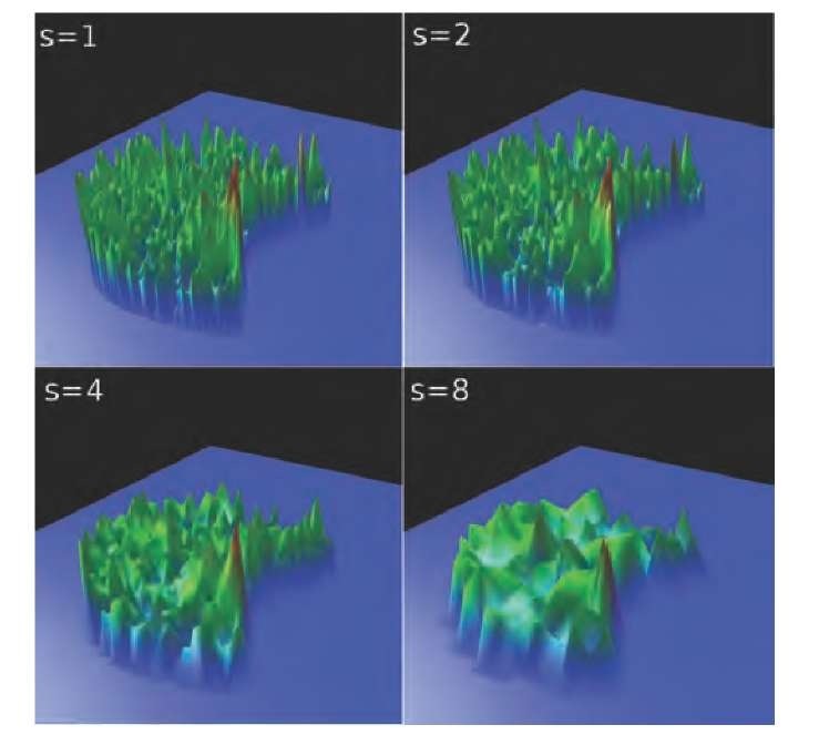
FIGURE 10.18 Four steps in the process of calculating the blanket dimension. Starting with the top left image, the landscape is drawn with one pixel per box (s = 1), whereas in subsequent iterations 4 pixels (s = 2), 16 pixels (s = 4), and 64 pixels (s = 8) are averaged. As a consequence, the elevation landscape becomes less jagged and the surface area decreases.

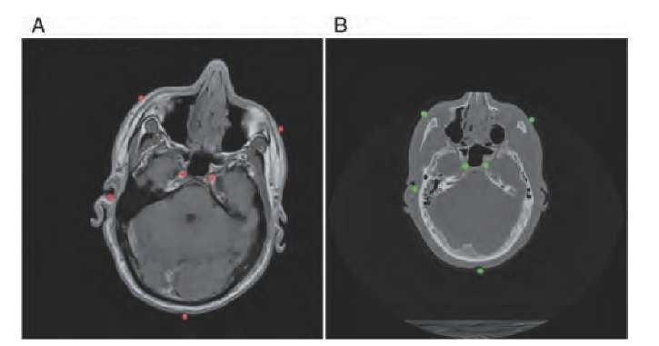
FIGURE 11.3 Matched but unregistered slices from the Visible Human data set. (A) shows a Ti>-weighted MR slice of the head, and (B) shows the corresponding CT slice. The images are mismatched in position, rotational orientation, and scale. Anatomy-based homologous fiducial markers (red in the MR image and green in the CT image) have been placed manually.

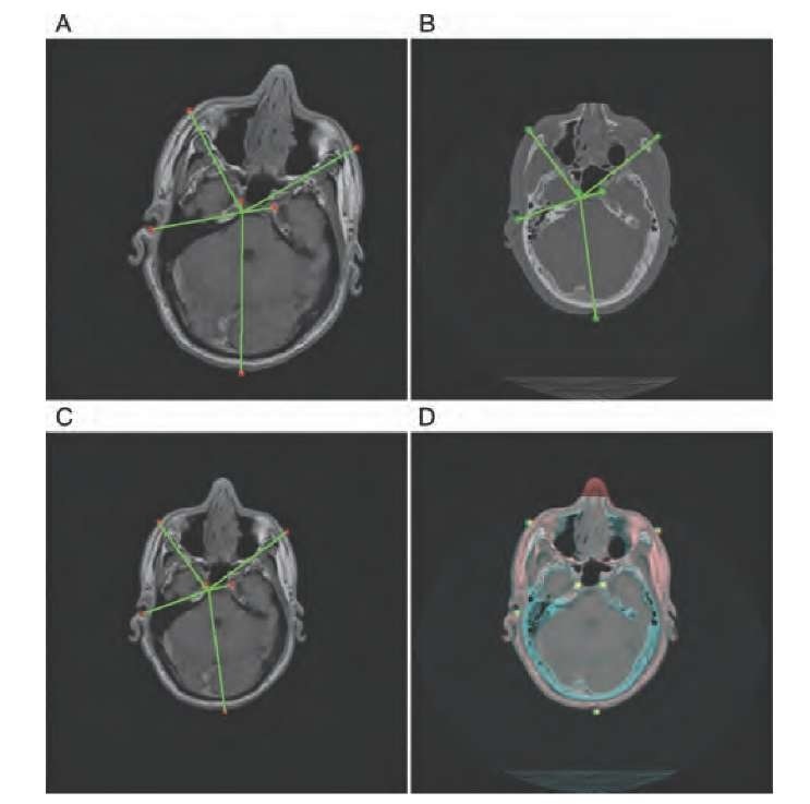
FIGURE 11.4 Registration process based on fiducial markers. First, the centroid of the markers is determined (green lines in A and B). Next, the centroids are brought in congruence with a translation operation. The angles of the green lines provide the necessary rotation angle, and the length ratio provides the scaling factor. After the transformation, the MR image (C) matches the CT image (B) in terms of position, rotation, and scale. It can be seen that the green lines, which connect the fiducial markers with the centroid, have the same length and orientation in (B) and (C). The images are then fused (D), with the MR image having a red tint and the CT image having a blue tint. A minor mismatch can still be seen; this mismatch cannot be corrected with rigid-body transformations.

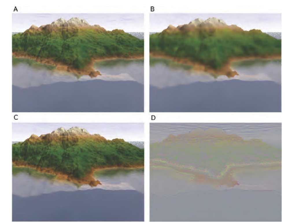
FIGURE 12.8 Demonstration of the effect of selective image information loss. Image A, subjected to an adaptive anisotropic diffusion lowpass filter, is strongly blurred (B). The loss of detail at high spatial frequencies is obvious. Conversely, when only the color (hue and saturation) information is blurred and the intensity information is left unaltered (C), almost no differences to the original image are detectable. The difference between images A and C is shown in image D.

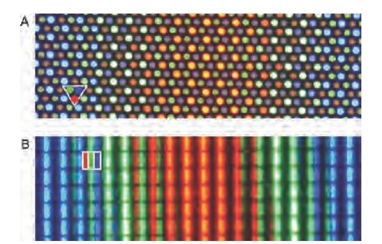
FIGURE 13.2 Demonstration of additive color generation. The images are magnified sections of photographs of a CRT screen (A) and a LCD screen (B), both displaying a color gradient blue-green-red-green-blue. In each image, one pixel is delineated (white triangle and square, respectively). Each pixel is approximately 0.25 mm in size. It can be seen that each pixel is composed of three components: red, green, and blue. Note that the camera that was used to take these photos has a high sensitivity for green, and the brightest green segments are overexposed.

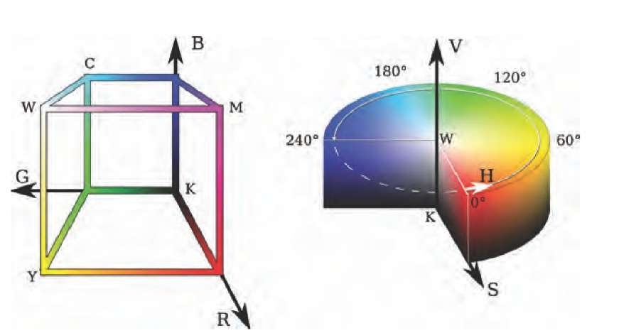
FIGURE 13.3 Graphical representations of the RGB and HSV color models. Each color represents one point inside the RGB cube, and its position is determined by the value of its R, G, and B components in Cartesian coordinates. Here, only the edges of the filled cube are shown. The edges of the cube give an example of the color gradients with black (k) and white (w) at diagonally opposite ends, and with the additive colors cyan (c), magenta (m), and yellow (y) at off-axis corners. The HSV model uses a cylinder coordinate system with the hue (H) as the angular component, the saturation (S) as the radial component, and the value (V, also known as intensity or brightness) as the axial component. The central axis of the cylinder covers the gray-value gradient from black to white.

FIGURE 13.4 Gray-scale image of a micro-CT cross section of a mouse femur (A) and three false-color representations (B-D). In (B), the color scheme called Rainbow [Equation (13.5)] was applied, in (C) the color scheme called Fire, and in (D) a color scheme called Terra. The graphs underneath the color images are the corresponding lookup tables (the x-axis is the image gray value and the y-axis is the color component value). Whereas smooth transitions were desired in images B and C, the Terra color scheme in image D introduces abrupt transitions, which cause the appearance of contour bands.