Adaptive Noise Reduction Part 2 (Biomedical Image Analysis)

Anisotropic Diffusion Lowpass Filter

Perona and Malik introduced a very powerful adaptive filter that operates by numerically simulating anisotropic diffusion.28 Image intensity values can be thought of as local concentrations caught inside the pixel. If pixel boundaries are thought of as semipermeable, the pixel intensity would diffuse over time into neighboring pixels of lower intensity (i.e., follow the negative gradient). This process is most dominant wherever high contrast exists between neighboring pixels, and the diffusion process would end after infinite time with all contrast removed. This type of diffusion follows the partial differential equation

By using g as a function of the local gradient, the diffusion speed g( VI) ■ VI becomes low at high local gradients (i.e., edges) and finds a maximum at—or, depending on the function g, near—the value of the constant K. The function g in Equation (5.12)

where I(x,y,t) is the image intensity, c is the diffusion constant, and A indicates the Laplacian operator. Equation (5.10) describes an isotropic diffusion process that leads to Gaussian blurring. The key to anisotropic diffusion is to introduce a locally adaptive diffusion constant c(x,y,t) which changes the diffusion equation to

where V indicates the gradient operator and div indicates the divergence operator. This diffusion constant needs to be chosen as a function of the local gradient28 with a function g that is monotonically falling and normalized to g(0) = 1. An example of a suitable function g is and the diffusion speedis shown qualitatively in Figure 5.5. The most interesting property of anisotropic diffusion, the enhancement of high-contrast edges, is related to the negative slope of the diffusion speed at high gradients.28 Despite the comparatively complex theory behind the anisotropic diffusion filter, a numerical approximation of the diffusion equation, and therefore its computer implementation, are surprisingly simple. Let us discretize the intensity gradient into the intensity difference of a pixel to its four neighbors:

FIGURE 5.5 Graphical representation of the functionin Equation (5.12) and the diffusion speed

Then the four directional components of the diffusion constant can be computed:

Finally, the partial derivative toward time in Equation (5.11) can be discretized with an iterative time-stepping loop where one step advances the diffusion by the time A t:

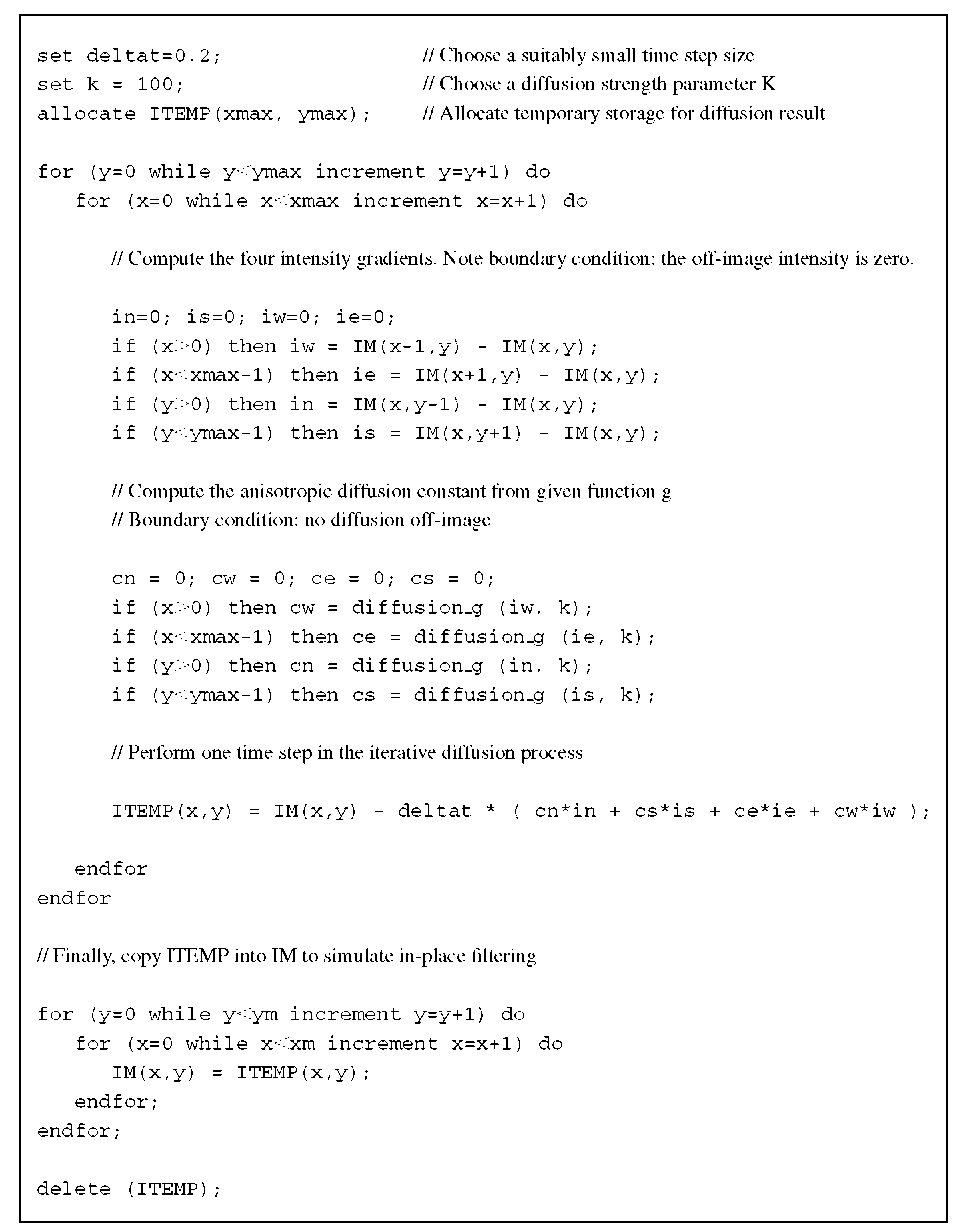
If a function g is defined [Equation (5.12), termed diffusion_g in the computer implementation] that returns a floating-point value g from the floating-point parameters grad_i and k, we arrive at the implementation described in Algorithm 5.2.

Algorithm 5.2 Anisotropic diffusion lowpass filter. Each execution of this algorithm performs one time step according to Equation (5.15). The input image is IM(x,y), and the diffused image is stored temporarily in ITEMP(x,y). Afterward, ITEMP is copied into IM so the diffusion is applied to the input image. This process needs to be repeated several times to achieve sufficient noise reduction.

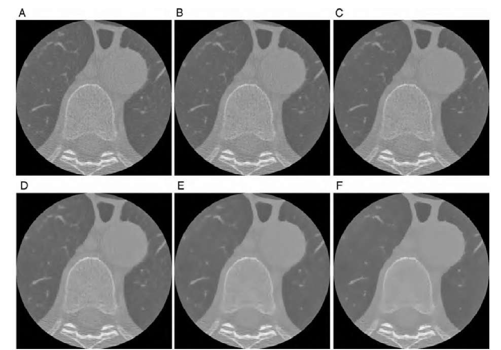
The parameter K, which determines the strength of the filter by determining where the negative diffusion gradient starts, and the number of iterations strongly determine the outcome of the filter. An optimum value of K and the optimum number of iterations are normally determined experimentally, although K can be made dependent on the noise component of the image,28 for example, by computing a histogram of the image gradient magnitude at each time step and selecting K to be the 90% quantile of the histogram. The main advantage of computing K in dependency of the noise component is the fact that one less parameter is arbitrarily chosen. Furthermore, as the noise component is reduced at higher iterations, K diminishes, and the filter strength diminishes as well. As a consequence, the number of iterations becomes less critical in determining the outcome. The automated selection of K is a major step toward an unsupervised anisotropic diffusion filter. The influence of the parameter K and the number of iterations are demonstrated in Figure 5.6.

A further option to fine-tune the filter is the choice of the function g. An alternative choice, the function g(VI) = exp(-V12/K2), exhibits a steeper drop-off at higher gradients and therefore preserves smaller detail than the function given in Equation (5.12). Finally, an improvement in the directional behavior can be achieved by including the diagonal neighbors in the diffusion equation.

FIGURE 5.6 Application of the anisotropic diffusion lowpass filter on the CT slice in Figure 5.3A. For the top row (A, B, C), the parameter K was set to 50 and the diffusion process was iterated 20, 50, and 100 times, respectively. In the bottom row (D, E, F), K was set to 100 and the diffusion process was iterated 20, 50, and 100 times, respectively. At a high number of iterations, the edge-preserving property of the filter becomes particularly apparent.

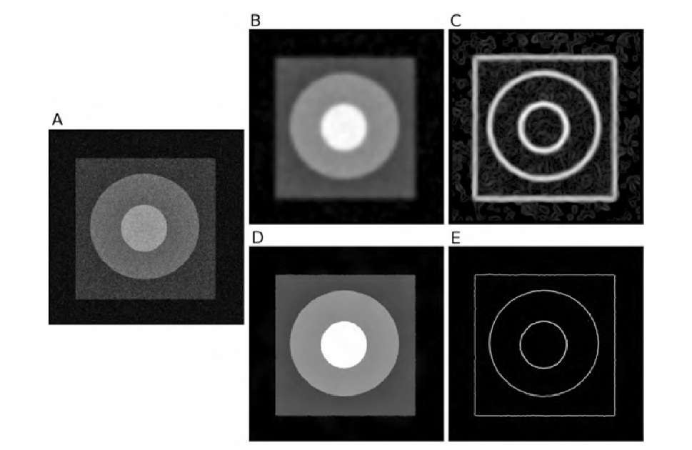
FIGURE 5.7 Application of anisotropic diffusion to denoise an image. The original image (A) consists of several areas of different gray values (range 0 to 255) with step transitions and superimposed Gaussian noise with a = 40. Repeated application of strong Gaussian blurring leads eventually to image B, where noise is widely smoothed, but the transitions are blurred, too. As a consequence, the application of an edge detector (Sobel operator) on image B yields fairly broad edges with considerable background texture (C). Anisotropic diffusion (10 iterations, K = 50 followed by 300 iterations, K = 12) not only removes the noise component completely but also preserves the step edges (D). The application of an edge detector on image D results in sharp edges that are only minimally distorted (E).

An example of the application of anisotropic diffusion in noise removal is shown in Figure 5.7, where conventional nonadaptive Gaussian blurring is compared with anisotropic diffusion. With extremely noisy images, such as Figure 5.7A, a suitable denoising approach needs to be determined experimentally. In this example, two stages of anisotropic diffusion were applied. For the first stage, K = 50 was selected but only 10 iterations were executed. This value of K is large enough to blur the boundary of the dark rectangle, but blurring is limited because of the low number of iterations. However, with the large value of K, the initial diffusion step considerably reduced the noise component. In the second step, a smaller value for K was chosen (K = 12), which prevented blurring of the lowest-contrast edge, and with the high number of iterations, the remaining noise was removed almost completely.

Adaptive Median Filters

Although averaging filters are effective for removing Gaussian noise, the median filter is more suitable for shot noise (also known as salt-and-pepper noise or impulse noise). Shot noise is characterized by pixels that assume the maximum or minimum image value with a certain probability. Images affected by shot noise typically occur when individual pixels are not covered in the image formation or reconstruction process. For comparison, additive noise affects every pixel by displacing its value by a random offset e. An image degraded by Gaussian noise can be modeled as

where g(x,y) is the degraded image, f (x,y) is the ideal image, and e(x,y) is the Gaussian noise component with zero mean and an image-specific standard deviation.

On the other hand, shot noise affects pixels only with a probability p, but an affected pixel will either assume the image’s maximum or minimum value. In 8-bit images, these pixels would be black [g(x,y) = 0] or white [g(x,y) = 255]. The degradation process can be modeled as

where n(x,y) is either black, or white, or a combination of black and white pixels with a different probability p2 for a black pixel. Therefore, an image that is affected by shot noise contains a number of white and black pixels.

A conventional, nonadaptive median filter sorts the values of a n x n neighborhood (most often a 3 x 3 neighborhood) and replaces each image value by the median of its neighborhood, thus eliminating runaway values such as black or white pixels. A locally adaptive median filter has been proposed38 in which the neighborhood is expanded as long as the median value is typical for its neighborhood. More specifically, for each pixel, a starting neighborhood of n x n is set: for example 3 x 3. For this neighborhood, the minimum, median, and maximum intensities (Imin, Imed, and Imax, respectively) are determined and the condition Imin < Imed < Imax is tested. If this condition is not satisfied, usually with either Imin = Imed or Imed = Imax (thus indicating that a likely runaway value exists in the neighborhood), the neighborhood is expanded. If a predetermined maximum neighborhood size is reached, the pixel remains unaffected; otherwise, the process is repeated. If, on the other hand, the condition Imin < Imed < Imax is satisfied, another test is performed; that is, Imin < I(x,y) < Imax. If this condition tests true, the central pixel I(x,y) is unlikely to be impulse noise, and the pixel remains unaffected. Otherwise, the central pixel I(x,y) is probably impulse noise and gets replaced by Imed. For large neighborhood sizes, the adaptive median filter retains edges and details better than a conventional median filter.

The center-weighted median filter (CWMF) was proposed by Ko and Lee18 as a weaker median filter with better edge-preserving properties than those of the conventional median filter. This attenuated median filter differs from the conventional median filter inasmuch as the neighborhood table, from which the median value is determined, is extended by w – 1 values and the central pixel value is repeated w times. An example is given in Figure 5.8. Depending on the value of w, the CWMF is less likely to replace a pixel by the neighborhood median value than by the conventional median filter. For this reason, the CWMF preserves edges, corners, and lines better than the conventional median filter does at the expense of lower filtering power. A locally adaptive combination of the CWMF and the median filter was proposed by Chen et al.11 and termed the tristate median filter, because the filter either replaces a pixel by the output of the median filter or by the output of the CWM filter, or leaves the pixel unchanged, depending on the local neighborhood properties.

FIGURE 5.8 Center-weighted median filter (CWMF). Shown is a sample neighborhood (left) and the nine neighborhood values sorted ascendingly (right, top). The median value of the neighborhood is 36. The CWMF extends the neighborhood list by repeating the central value w = 4 times (right, bottom). In this example, the central pixel value and the median value coincide. The CWMF is less aggressive than the conventional median filter.

More specifically, for each pixel f(x,y), the median filter outputfmed(x,y) and the CWMF output f CWMF(x,y) are determined. A threshold value T is provided for the decision mechanism, and the final filtered image value g(x,y) is determined through

whereThe threshold value T determines the strength of the filter. Setting T = 0 leads to the conventional median filter. A very large threshold value leaves the image unmodified. Threshold values in between yield the adaptive behavior, and a smaller threshold leads to a stronger filter action. The choice of a suitable threshold value needs to be determined experimentally, ideally with a training set of images where the mean-squared error (or any other distance) is minimized.

The idea of adaptive median filters can be taken further to allow for a correction step between two successive applications of a median filter. The principle behind the correction of a median filter step lies in the filter’s possible types of error: A median filter can either miss a corrupted pixel, correct a noncorrupted pixel, or replace a pixel by a new value that has a larger distance to the (unknown) uncorrupted pixel than the original corrupted pixel. This third type of error, referred to as overcorrection error, is minimized by the filter proposed by Xu et al.41 The first step of this two-stage filter is the application of a conventional median filter, a CWM filter, or any other adaptive rank filter such as the adaptive median filters described in previous sections. In preparation of the corrective step, a binary image is created, which contains white pixels (1′s) where the original image and the median-filtered image differ, and which contains black pixels (0′s) where they don’t. Let us denote the input image I, the median filter output F, and the black-and-white image that indicates pixels that were replaced by the median filter D. To identify those pixels of D that have probably been overcorrected, an adaptive processor is proposed that creates another image E, which is a subset of D and contains 1′s only for those pixels that are identified as overcorrected. The adaptive processor operates row by row and processes one row of D as follows:

Step 1. Choose two parameters a and b that determine the filter action. Step 2. Count the probability of white pixels in all rows n. Denote this probability w(n). w(n) is therefore a column vector, and the mean and standard deviation of w(n), denoted ^(w) and a(w), can be computed. Step 3. Compute two threshold values i = aa(w) and k = ^(w) – ba(w). In addition, copy the first median-filtered image F into G. Step 4. For each row n, execute steps 5, 6, and 7 only if w(n) > ^(w) + r|. Step 5. For row n, determine the number K of pixels probably overcorrected using K = w(n) — ^(w) + ba(w) = w(n) – k. Step 6. In row n, compute the error vector e as the element-by-element squared difference of row n in I and F. Step 7. Find the K smallest values in e and revert the action of the median filter for the corresponding elements in G (i.e., replace the corresponding elements in G by the original elements from I). Step 8. After all rows have been processed, compute E as the binarized difference image between F and G in the same manner as D was computed from F and I. In this way, E contains 1′s on all positions where the action of the first median filter was reverted.

In the second stage of this filter, G is subjected to a conditional median filter step: A pixel in G may be changed as a result of the median filter only if the corresponding element of E is zero (in other words, if the pixel was not reverted by the adaptive processor). The output of the conditional median filter step G is the output of the entire adaptive filter.

The filter algorithm can further be simplified if the reversal of overcorrected pixels takes place directly in D and D serves as decision mechanism whether to use pixels from I or F in the final filtered image. In this case, E and G are no longer needed. Although the filter as proposed by Xu et al.41 preserves some detail over the nonadaptive median filter, its line-by-line processing sequence makes the filter action highly orientation-dependent. Furthermore, the optimum parameters a and b are not intuitively easy to find. The filter could be improved by examining the median filter correction statistics in a square local neighborhood rather than in a horizontal line.