Adaptive Noise Reduction Part 1 (Biomedical Image Analysis)

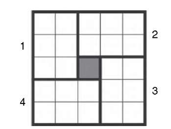
Noise reduction is one of the most important image processing steps, particularly in biomedical image processing. Noise is broadly distributed over the frequency spectrum of the image. The conventional approach to reducing noise is the application of a blurring filter (e.g., Gaussian smoothing or lowpass filtering in the frequency domain). Unfortunately, degradation of high-frequency components—edges and texture details—is an inevitable consequence of the blurring process. For this reason, many methods and algorithms have been developed that act more strongly in flat image regions than near edges. Generally, adaptive noise reduction results in nonlinear filters and filters that are defined only algorithmically. A good example for a nonlinear, edge-preserving noise reduction is the Kuwahara filter, although it is not an adaptive filter. The Kuwahara filter can be explained by the definition of four neighborhood areas of the central pixel (dark gray) in Figure 5.2. Four adjacent, nonoverlapping regions of the local window are examined and the central pixel value is replaced by the mean value of the pixels in the region with the lowest variance. The window size (in this example, 5 x 5, which leads to four six-pixel regions) can be freely selected. The averaging operation, in combination with choosing the lowest-variance quadrant, is responsible for noise reduction. If an edge runs through the window, the Kuwahara filter generally picks a region that does not contain the edge, because the edge causes a high variance where it intersects one of the four regions. The Kuwahara filter illustrates the basic idea behind edge-preserving noise-reduction filters, but superior adaptive filters have been developed.

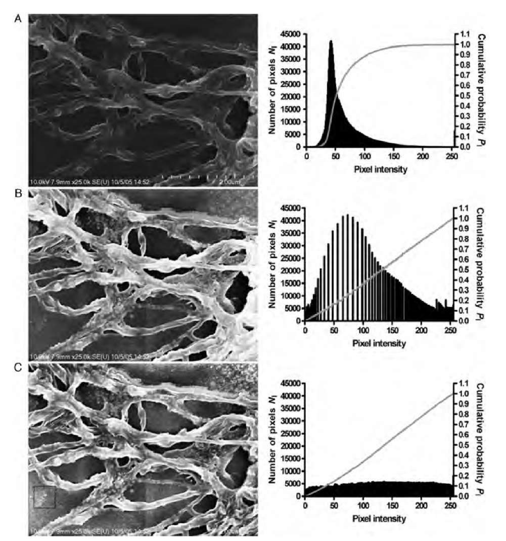
FIGURE 5.1 Global and locally adaptive histogram equalization. Image A shows a scanning electron microscope (SEM) image of grown collagen fibers. The histogram reveals an emphasis on dark shades with few bright image values. Global histogram equalization (B) enhances the contrast by brightening mid-gray pixels, but the histogram shows that the available value range is not fully used. Locally adaptive histogram equalization (C) leads to optimized contrast in each region. The neighborhood size in image C is indicated by a black rectangle near the bottom left corner.

FIGURE 5.2 Pixel neighborhood definition for the Kuwahara filter in the example of a 5 x 5 neighborhood. The central pixel is replaced by the average value of the six pixels in the region (1 to 4) that has the lowest variance.

Adaptive Minimum Mean-Squared-Error Filter

A simple and widely used locally adaptive noise reduction filter is the minimum mean-squared-error filter. It is based on variable-strength blurring to balance a strong filter action in flat regions with a weaker filter action in the presence of edges. If we assume that the noise component of the image is known and has an overall variance aN we can intuitively demand that a locally adaptive filter acts strongest wherever it finds a local variance a£c close to the global noise variance a^. In the presence of edges or other image features, the local variance can be expected to be higher than aN, and the adaptive filter reduces the strength of its blurring action. In its simplest implementation, the minimum mean-squared-error filter can be described by20

where any pixel value I (x,y) is substituted for by a new value I’(x,y) that depends on the original intensity value, the local variance a^c [computed inside an M x M

Equation (5.4) is a one-pass equation that allows us to compute the local mean value and the local variance in the same loop over the square region by summing up the image values and the squared image values. It can be seen from Equation (5.3) that in areas of low local variance (ct^ ^ ct^) the new image value is close to the local average value, whereas in areas with high local variance (ct^ > ct^), the filter does not strongly modify the original intensity value. For practical application of the minimum mean-squared-error filter, the global variance can be approximated by the smallest local variance encountered:

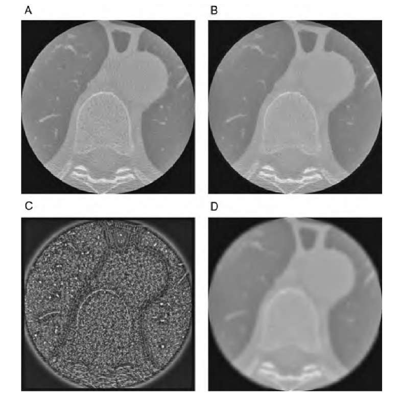
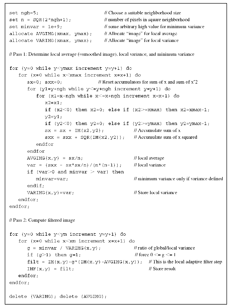
This assumption implies that areas with low image contrast exist and that the noise variance is the same in all regions of the image. An example is shown in Figure 5.3, where a CT image of the lung is subjected to a conventional Gaussian blurring filter and a local adaptive filter following Equation (5.3). The difference image (panel C) shows the noise removed, but it also shows dark areas along edges, indicating that the filtered image does not differ from the original image in those regions. A possible implementation is shown in Algorithm 5.1.

The filter described in Algorithm 5.1 is weaker than the smoothing filter that is used to compute I(x,y) in Equation (5.3). With the practical implementation described here, the minimum variance that is used for ct^ may result in a very small value, making the overall effect of the filter even weaker. One possibility is to use a histogram-based approach to determine o^: for example, computing the histogram of VARIMG in Algorithm 5.1 and choosing ctN from the 5% or 10% quantile of the histogram. With this more refined method, the choice of ct^ becomes more robust against image anomalies that violate the assumption of homogeneously distributed noise. Further improvements in the algorithm are possible by implementing a circular neighborhood. Also, the averaged image intensity II could be computed more advantageously by using a Gaussian rather than a box kernel.

The major disadvantage of this adaptive filter is the poor noise reduction near edges, which is a component of the filter design. Nonetheless, modification of this filter for improved noise reduction near edges is possible.32 An edge detector can be used to determine if an edge exists in the local neighborhood: for example, by application of the Sobel operator or Canny edge detector with subsequent thresholding. If an edge exists, the local window can be split into two regions under the assumption that square neighborhood with l = M/2 - 1, as defined in Equation (5.4)], the global noise variance ct^, and the mean intensity value I(x,y) in the neighborhood: the edge is straight. Computation of the local variance is then restricted to that side of the edge where the central pixel is located. Alternatively, the filter can be applied iter-atively with an update of aN2 after each iteration. Since aN2 is reduced after each filter pass, the iterative application of the adaptive minimum mean-square filter converges.

FIGURE 5.3 Application of a locally adaptive noise removal filter to a CT image of the lung, which contains a strong component of pseudostructure (A). The filtered image (B) shows good smoothing in homogeneous areas (lung, aorta), while the edges are retained. This is illustrated further in image C, the absolute difference of the original and filtered image, in other words, the component removed from image A by filtering. Dark regions in image C represent regions where the adaptive filter did not change the image. Most prominently, the lung contour can be seen as a dark line. Image D shows the application of conventional Gaussian blurring to image A. Although the noise largely been removed, the edges have deteriorated, and detail inside the lung has been lost.

Adaptive Bilateral Filter

Using a different formulation, the adaptive bilateral filter by Zhang and Allebach42 also reduces noise while preserving edges. The adaptive bilateral filter is based on the convolution of the noisy image with two Gaussian kernels, one of which is adaptive.

Algorithm 5.1 Adaptive minimum mean-square filter. The input image is IM(x,y), and it is assumed that reading IM outside its defined area (0 to xmax-1 and 0 to ymax-1) returns defined values. The algorithm performs two passes. In the first pass, the local average, local variance, and the minimum variance are determined, and in the second pass, the actual filtering takes place, resulting in the filtered image IMF(x,y) .

The convolution kernel contains two exponential terms that describe two Gaussian functions. The first exponential term is a two-dimensional Gaussian function with the standard deviation ad2, and the second exponential term represents a Gaussian function of the image gradient. These exponential terms are referred to as the domain and range filters, respectively, and their combination was given the name bilateral filter. With a very large value of ar, the bilateral filter degenerates into a conventional Gaussian blurring filter with a standard deviation of ad. In the presence of edges, the second term causes a directional distortion of the Gaussian kernel: The kernel elongates along the edge, and averaging occurs predominantly along the edge and less strongly perpendicular to the edge. This behavior is the basis for the edge-preserving properties of the bilateral filter. a r is a variable parameter, which can be used to control the width of the filter. With large values of ar, the range filter will assign approximately equal weights for each pixel in the window, and the filter behaves predominantly like a Gaussian blurring filter. With small values for ar, the range filter dominates the bilateral filter and the adaptive behavior is more pronounced.

The final parameter, £ (x,y), is responsible for the adaptive behavior. If £ (x,y) = 0, the filter is nonadaptive and corresponds to the conventional bilateral filter proposed by Tomasi and Manduchi.37 To obtain adaptive properties, including sharpening of the edges, the maximum (Imax), mean (Imean), and minimum (Imin) values of the pixel neighborhood need to be determined. The difference between any given pixel I(x,y) and the neighborhood mean value Imean can be defined as A (x,y) = I(x,y) – Imean. The behavior of the filter near edges is now determined by three preferred choices of £ (x,y):

1. Shifting the image values in the neighborhood window toward Imean by choosing £ (x,y) = – A (x,y) causes edges to blur, and the filter has an overall smoothing character.

The general filter equation is a convolution of the degraded (noisy) image I(x,y) with a kernel h(x,y,m,n) to obtain enhanced image I’ through where 2l – 1 is the square neighborhood size. The kernel h is computed through

and the normalization factor r(x,y) through

2. Shifting the image values in the neighborhood window away from Imean by choosingcauses noise reduction combined with edge sharpening.

3. Separating the image values and shifting them toward Imax and I^n by choosing according to the following equation depending on the sign of causes a drastic sharpening effect with a strong steepening of the edges:

The adaptive bilateral filter is best demonstrated by using a synthetic test image. Figure 5.4A shows some geometrical structures that were blurred and spoiled with additive Gaussian noise (a = 10) (Figure 5.4B). Figure 4.4C demonstrates the effect of the conventional bilateral filter (l = 9, ad = 2, and ar = 20), which strongly reduces noise while not blurring the edges further. The adaptive bilateral filter, on the other hand, restores some of the edge sharpness (Figure 5.4D). With multiple applications of the adaptive bilateral filter, image restoration can be improved further (Figure 5.4E).

FIGURE 5.4 Demonstration of the operation of the adaptive bilateral filter. A test image (B) was created from a synthetic image (A) by performing Gaussian blur and adding Gaussian noise with a standard deviation of 10. The nonadaptive, conventional bilateral filter (£ = 0) already shows good noise suppression while retaining edge contrast (C). Application of the adaptive bilateral filter [£ (x,y) = +A (x,y)] leads to image D, with similarly good noise suppression but an additional restoration of edge sharpness. Image E was created with two successive applications of the adaptive bilateral filter. Images F and G illustrate the composition of the kernel h: the white rectangle in image B indicates the position of the two kernels. Image F is the nonadaptive domain filter kernel, and image G is the adaptive bilateral kernel. It can be seen that the kernel contains zero values on one side of the edge, averaging only values on that side of the edge where the central pixel lies.

Figure 4.4F and G illustrate the kernel h. This kernel is computed at the location of the white rectangle in Figure 5.4B, and Figure 5.4F shows the Gaussian domain filter kernel, which is nonadaptive. The combination of the range and domain kernels h is shown in Figure 5.4G. It can be seen that the kernel becomes asymmetric along the edge as a consequence of the range filter: Pixels across an edge lose their influence on the kernel; therefore, the averaging takes place on pixels along one side of an edge.

A disadvantage of the adaptive bilateral filter is the empirical nature of the optimum values for CTd and o>, and one of the main disadvantages is that the value of A, used to compute offset £ in the range filter, is highly noise-dependent. Furthermore, the optimum choice of the parameters ctd and ctr are dependent on the gray-value range of the image. To optimize this filter, some experimentation is therefore needed. Even more advantageous is the use of a training set to optimize the filter parameters.42