Technique of Statistical Validation of Rival Models for Fatigue Crack Growth Process and Its Identification (Statistics Inference) (Analytical and Stochastic Modeling) Part 2

Test for the Operational Validity

The test of H0(k) versus H1(k), based on vn(k), is given by

where h(k)>0 is a threshold of the test which is determined for a prescribed level of significance a(k) as

of the F-distribution with 1 and n-1 degrees of freedom. When the parameteris unknown, it is well known that no the uniformly most powerful (UMP) test exists for testing H0(k) versus H1(k). However, it can be shown that the test (50) is uniformly most powerful invariant (UMPI).

It will be noted that the null distribution of vn(k) is F-distribution with 1 and n-1 degrees of freedom for such distributions of z(k) as the Cauchy distribution, f-distribution [17].

Fatigue Crack Growth Process Identification

When there are the m specified rival models, the problem is to identify the observable fatigue crack growth process with one of these models. If there is the possibility that the observable process cannot be identified with one of the m specified rival models, it is desirable to recognize this case too.

If (m-1) rival models are eliminated by the above test, then the remaining model (say, kth) is the one with which the observable fatigue crack growth process may be identified.

If all rival models are eliminated from further consideration, we decide that the observable process cannot be identified with any of the m specified rival models.

If the set of rival models not yet eliminated has more than one unit, then we declare that the observable stochastic process may be identified with rival model k* if

is the set of rival models not yet eliminated by the above

is the set of rival models not yet eliminated by the above model validation test.

Example

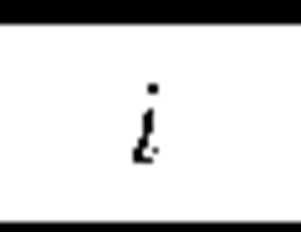
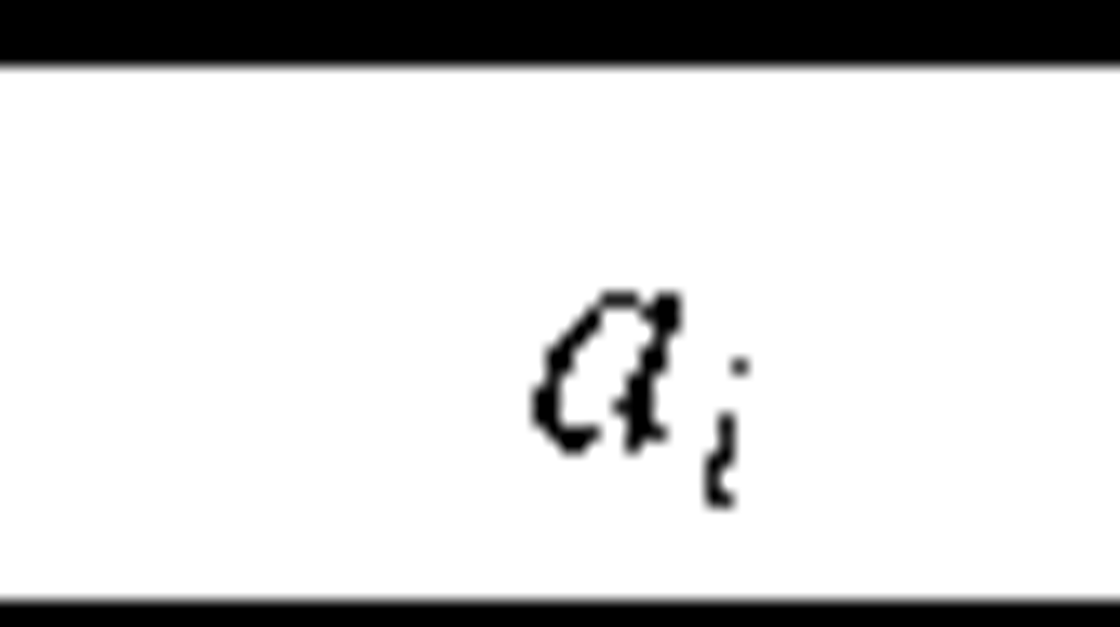
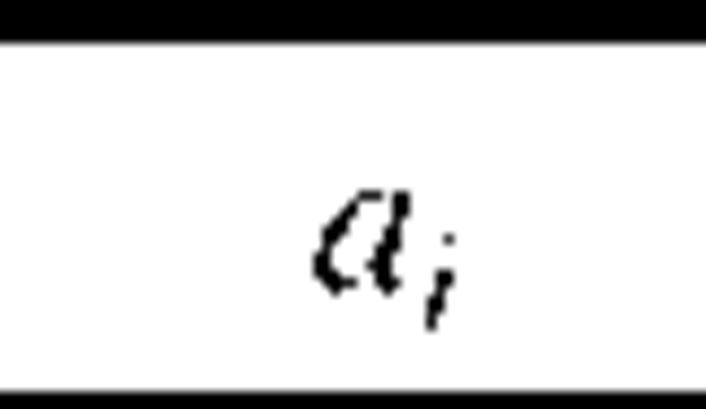
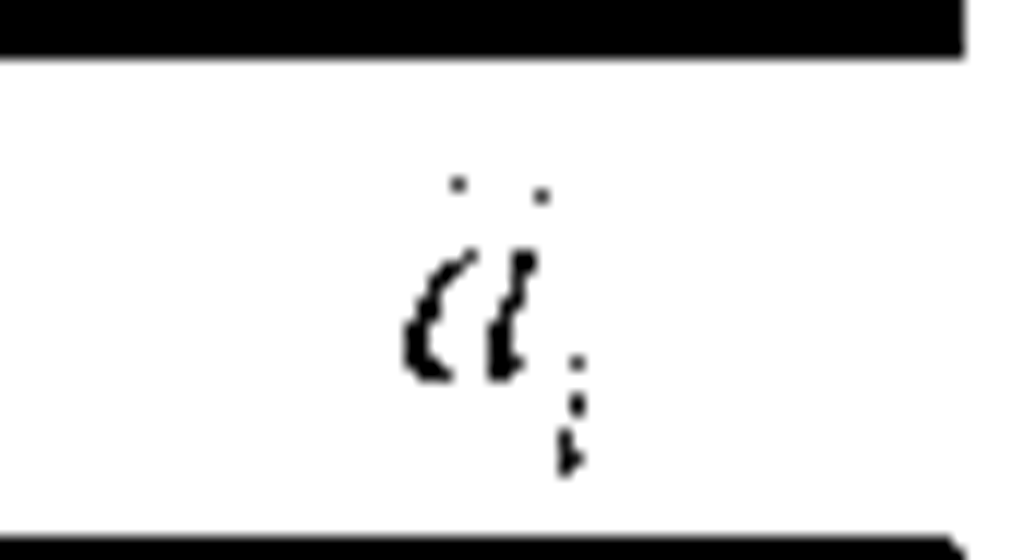
Consider the data of fatigue crack growth process in upper longeron of RNLAF F-16 aircraft (Table 2, where t is the flight hours, at is the crack size (in mm)).

Table 2. The data of fatigue crack growth process in upper longeron of RNLAF F-16 aircraft

i	ti	a	i	ti	a	i	ti	a	i	ti	a
1	500	0.20	4	0.32	2000	7	0.50	3500	10	1.60	5000
2	1000	0.25	5	0.35	2500	8	0.65	4000	11	2.60	5150
3	1500	0.30	6	0.40	3000	9	1.00	4500	12	4.00	5300

It is assumed that a0=0.18 for f0=0.

Validation of Models 1 and 2 for the Fatigue Crack Growth Process

Conceptual Model Validation. Using the data of Table 2, we have:

Model 1. It follows from (19), (20) and (21)),

It follows from (27), (28), (30) and (53),

Thus, there is not evidence to rule out the normality assumption (25). Model 2. It follows from (23), (24) and (21),

It follows from (27), (29), (30) and (55),

Thus, the normality assumption (26) is not rejected.

Operational Model Validation. Using (11) and (53), we have the results of the fatigue crack growth process prediction by means of Model 1:

which are given in Table 3.

Table 3. The results of the fatigue crack growth process prediction by means of Model 1

1	0.20	0.203	4	0.32	0.315	7	0.50	0.582	10	1.60	1.622
2	0.25	0.232	5	0.35	0.377	8	0.65	0.765	11	2.60	1.889
3	0.30	0.269	6	0.40	0.462	9	1.00	1.065	12	4.00	2.236

Let

Based on (44) and the data of Table 3, we find (for n=12, a=0.05)

Using (12) and (55), we have the results of the fatigue crack growth process prediction by means of Model 2:

which are given in Table 4.

Table 4. The results of the fatigue crack growth process prediction by means of Model 2

i	ai	ai	i	ai	ai	i	ai	ai	i	ai	ai
1	0.20	0.201	4	0.32	0.357	7	0.50	0.500	10	1.60	1.691
2	0.25	0.226	5	0.35	0.384	8	0.65	0.657	11	2.60	1.961
3	0.30	0.290	6	0.40	0.427	9	1.00	0.919	12	4.00	3.561

Let

Based on (44) and the data of Table 4, we find (for n=12, a=0.05)

It follows from (59) and (62) that the rival models (Model 1 and Model 2) pass the operational validity test (50).

Identification of the Fatigue Crack Growth Process

Using the data of Tables 3 and 4, we find from (52):

It follows from (63) that the fatigue crack growth process may be identified with Model 2.

Planning Inspections in Service of Fatigued Structures

Now Model 2 can be used for planning in-service inspections of fatigued structures. In this case a sequence of inspections is determined as follows.

where Tj is the time of the jth inspection,

It will be noted that the jth inspection is assigned if

Conclusion

This paper addresses the analysis aspects of stochastic crack propagation process. The technique can easily be implemented for practical applications In addition to the statistical dispersion of the crack growth rate, the statistical dispersion of the initial flaw size is very significant and it should be accounted for in the reliability analysis of structural or mechanical components. Given the distribution of the initial flaw size, methodologies to account for both the crack growth variability and the initial flaw size variability have been available in the literature. However, the technology for establishing the initial flaw size distribution is still a subject of research.