Abstract
The development of suitable models of stochastic crack growth process is important for the reliability analysis of fatigued structures as well as the scheduling of inspection and repair/replacement maintenance. Based on modifications of the solution of the deterministic differential equation for the crack growth rate, where a stochastic nature of this rate is expressed by a random disturbance embedded in the solution of the differential equation, the simple stochastic models are presented for practical applications. Each of these models represents a stochastic version of the solution of the Paris-Erdogan law equation. The models take into account the random disturbance parameters while maintaining the simplicity and advantages of the Paris-Erdogan law equation. A technique is proposed in order to find the appropriate model for crack growth behavior from the family of rival models and test its validity in the light of experimental results. The model analysis technique can be implemented easily using deterministic crack growth analysis results and estimates of the statistics of the crack growth behavior. The solution of the deterministic differential equation associated with the stochastic model gives us the crack exceedance probability as well as the probability of random time to reach a specified crack size. Once the appropriate stochastic model is established, it can be used for the fatigue reliability prediction of structures made of the tested material. An illustrative example is given.
Keywords: Fatigue crack growth process, models, validation, identification.
Introduction
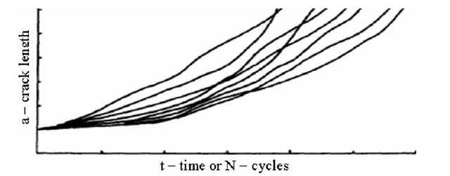
Models for fatigue crack growth process have been the subject of many papers published in the last 50 years. These span from simplified models (such as in [1]) to more advanced models (such as in [2]). Some of the models are based on the micro structure and some are based on the analysis of experimental data. Others are based on the theory of elasticity and use available experimental data for verification. Naturally it is beyond the scope of this paper to quote the enormous number of available works. The experimental work described in most of these papers shows that the size of the crack developed under repeated loads is of a random nature, although a repeated trend is observed. This was apparent even for the experiments carried out with tightly controlled laboratory settings under deterministic external loads. The measurement of crack size as a function of loading cycles (or time as an interchangeable parameter) has the general form shown in Fig. 1.
Fig. 1. Curves for crack size as a function of time or cycles
The curves are characterized by two features: (i) a non-linear increase in crack size with increased number of loading cycles (or time); (ii) intermingling of the curves for different "identical" specimens. Five series of experimental test results are repeatedly quoted in the literature: Noronha et al. [3] in which two sets of experiments are presented, Virkler et al. [4], Ghonem and Dore [5], and Wu and Ni [6]. From the nature of the phenomena and from the results quoted in these references and many others it can be seen that a good prediction of the behavior of the crack growth process must be given by a stochastic rather than a deterministic model. There is, therefore, a need to develop a probabilistic fracture mechanics framework for the modeling of fatigue crack growth in fatigued structures.
Probabilistic or stochastic models for crack growth were suggested by many investigators in the last 50 years. These include evolutionary probabilistic models (Markov chain, Markov diffusion models), cumulative jump models (Poisson process, birth process, jump-correlated model) and differential equation models. A comprehensive summary of the state of the art, with an excellent list of references, is given in ref. [7]. Each of the models may be the most appropriate one to depict a particular set of fatigue growth data but not necessarily the others. All models can be improved to depict very accurately the growth data but, of course, it has to be at the cost of increasing computational complexity. Yang’s model [8] and the polynomial model [9] are considered more appropriate than the Markov chain model [2] by some researchers through the introduction of a differential equation which indicates that fatigue crack growth rate is a function of crack size and other parameters. Unfortunately, they are mathematically too complicated for fatigue researchers as well as design engineers. A large gap still needs to be bridged between the fatigue experimentalists and researchers who use probabilistic methods to study the fatigue crack growth problems.
The models which are mainly used in practical engineering applications are the differential equation models. The methods by which the differential equation for the behavior of a stochastic structure due to crack growth is treated and the probability of failure of the structure is calculated can be divided into three major families:
(1) Use of the deterministic differential equation for the crack growth rate, while assuming that different parameters in this equation are random variables. Examples of this family are presented in [10-12]. This family is denoted by RV (Random Variables).
(2) Use of a modified differential equation for the crack growth rate, where a stochastic nature of this rate is expressed by a random process. Examples of this family are presented in [13]. This family is denoted by RP (Random Process).
(3) Use of a modified solution of the deterministic differential equation for the crack growth rate, where a stochastic nature of this rate is expressed by a random disturbance embedded in the solution of the differential equation. Examples of this family are presented in [11]. This family is denoted by RD (Random Disturbance).
In this paper, a technique is proposed in order to find the appropriate model for crack growth behavior from the RD family of rival models and test its validity in the light of experimental results. The implications of the results are then discussed for the identification of fatigue crack growth process.
Formulation of Models for the Fatigue Crack Growth Process
Deterministic Models for the Fatigue Crack Growth Process
With the application of fracture mechanics concepts to fatigue failure and the development of sophisticated crack detecting techniques, the crack propagation data can be obtained in terms of crack length (a) and number of cycles (N). In most cases, fatigue crack growth rate data in fatigued components are assumed to follow the Paris-Erdogan law [1]. This is given by:
where da / dN is the fatigue crack growth rate,![]() is the stress intensity factor range, C is the Paris coefficient and m is the Paris exponent. Both C and m are generally considered to be material constants for a given microstructural condition and composition. The stress intensity factor range,
is the stress intensity factor range, C is the Paris coefficient and m is the Paris exponent. Both C and m are generally considered to be material constants for a given microstructural condition and composition. The stress intensity factor range,![]() can be expressed in its usual form as:
can be expressed in its usual form as:
where F is a geometrical function, Aais the stress range, and a is the crack length. We may now substitute (2) into (1) to obtain the following expression:
Setting
(1) may now be expressed as:
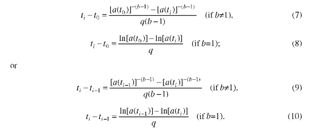
in which q and b are constants to be evaluated from the crack growth observations. The independent variable t can be interpreted as stress cycles, flight hours, or flights depending on the applications [14]. It is noted that the power-law form of![]() at the right hand side of (5) can be used to fit some fatigue crack growth data appropriately and is also compatible with the concept of Paris-Erdogan law. Separating variables in (5), the service time for a crack to grow from size a(t0) (or
at the right hand side of (5) can be used to fit some fatigue crack growth data appropriately and is also compatible with the concept of Paris-Erdogan law. Separating variables in (5), the service time for a crack to grow from size a(t0) (or ![]() can be found by performing the necessary integration between limits:
can be found by performing the necessary integration between limits:
to obtain (for i=1, …, n):
Thus, we have the two deterministic models for the fatigue crack growth process. 2.2 Stochastic Models for the Fatigue Crack Growth Process
In this paper, we consider stochastic version of the above deterministic models (7) and (9), respectively,
and
where![]() is a random disturbance,
is a random disturbance,![]() It will be noted that for typical aircraft metallic materials, an initial discontinuity size a(t0) (for f0=0) found through quantitative fractography is approximately between 0.02 and 0.2 mm. Let us assume that
It will be noted that for typical aircraft metallic materials, an initial discontinuity size a(t0) (for f0=0) found through quantitative fractography is approximately between 0.02 and 0.2 mm. Let us assume that![]()
Then the crack exceedance probability, i.e., the probability that crack size at will exceed any given (say, maximum allowable) crack size a’ can be derived and expressed either as (for Model 1):
where 0(.) is the standard normal distribution function; in this case, the conditional probability density function of at is given by
or as (for Model 2):
in this case, the conditional probability density function of at is given by
These models allow one to characterize the random properties that vary during fatigue crack growth.
Conceptual Model Validation
Conceptual model validation is defined as determining that the theories and assumptions underlying the model are correct and that the model representation of the problem entity is "reasonable" for the intended purpose of the model. For the above stochastic models: Model 1 and Model 2, the conceptual validation consists in the following.
Statistical Estimation of the Unknown Parameters
Model 1. Let us assume that the parameters b, q and a of the crack exceedance probability (13) are unknown. Given the data describing a single crack, say a sequence![]() it is easy to construct a log-likelihood using the density given by (14) and estimate the parameters b, q and a by maximum likelihood. The log-likelihood is
it is easy to construct a log-likelihood using the density given by (14) and estimate the parameters b, q and a by maximum likelihood. The log-likelihood is 
Inspection shows that this differs from the standard least-squares equation only in the term -bZlna, where the subscript i has been dropped. The likelihood estimators are obtained by solving the equations
In this case the equations have no closed solution. However, it is easy to see that the estimators for q and a given b are the usual least-squares estimators for the coefficients in (18) conditioned on b,
and on substituting these back in the log-likelihood gives a function of b alone,
Thus the technique is to search for the value of b that maximizes L(b) by estimating q and a as functions of b and substituting in L(b). In this study a simple golden-section search worked very effectively.
Model 2. In the same manner as for Model 1, we obtain the log-likelihood (from (16))
and the estimators for q and agiven b,
Substituting these back in the log-likelihood (22), we obtain (21) as a function of b alone. Then the statistical estimates of the unknown parameters b, q and a we find from maximization of L(b) (21).
Goodness-of-Fit Testing for the Normality Assumption
Model 1. The normality assumption is
Model 2. The normality assumption is
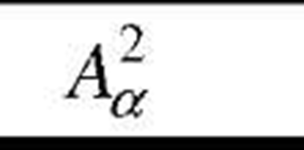
Of the many quantitative goodness-of-fit techniques suitable in this case (e.g.: Kolmogorov-Smirnov, Anderson-Darling, Shapiro-Wilk, von Mises), we prefer the Anderson-Darling test because it is more sensitive to deviations in the tails of the distribution than is the older Kolmogorov-Smirnov test. The Anderson-Darling statistic (A2) is defined as
where
and
The null and the alternative hypotheses are: H0: the data follow the specified distribution; HA: the data do not follow the specified distribution. The above formula needs to be modified for small samples,
and then compared to an appropriate critical value from Table 1 [15].
Table 1. Critical values for
 |
0.1 |
0.05 |
0.025 |
0.01 |
 |
0.631 |
0.752 |
0.873 |
1.035 |
The hypothesis regarding the distributional form is rejected at the chosen 2 2 significance level a if the test statistic, Ainod , is greater than the critical value Aa obtained from Table 1. The fixed values of a (0.1, 0.05 etc.) are generally used to evaluate the null hypothesis H0 at various significance levels. A value of 0.05 is typically used for most applications, however, in some critical industries, a lower a value may be applied.
Operational Model Validation
Operational model validation is defined as determining that the model’s output behavior has sufficient accuracy for the model’s intended purpose over the domain of the model’s intended applicability.
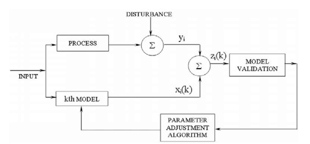
Suppose that we desire to validate a kth rival stochastic model of the fatigue crack growth process (see Fig. 2).
Fig. 2. Model validation scheme
Let xi(k) and yi be the ith observation of the response variable of the kth model and the process under study, respectively. It is assumed that all observations, xi(k), yi, i=1(1)n, are independent of each other, where n is a number of paired observations. Let![]() , be paired comparisons leading to a series of differences.
, be paired comparisons leading to a series of differences.
Thus, for testing the validity of a rival model of a real, observable stochastic process, it can be obtained and used a sample of n independent observations z(k)=fe(k), … , zn(k)). Each sample z(k), ke{1, … , m}, is declared to be realization of a specific stochastic process with unknown parameters. It is assumed in this paper that z,(k) (i=1, ., n) are normal random variables.
Hypotheses for Testing the Operational Validity
In this paper, for testing the operational validity of the kth rival model of a real, observable process, we propose a statistical approach based on the generalized maximum likelihood ratio. In using statistical hypothesis testing to test the validity of a rival model under a given experimental frame and for an acceptable range of accuracy consistent with the intended application of the model, we have the following two hypotheses:
H0: Model is valid for the acceptable range of accuracy under a given experimental frame; (31)
H1: Model is invalid for the acceptable range of accuracy under a given experimental frame.
There are two possibilities for making a wrong decision in statistical hypothesis testing. The first one, type I error, is accepting the alternative hypothesis H1 when the null hypothesis H0 is actually true, and the second one, type II error, is accepting the null hypothesis when the alternative hypothesis is actually true. In model validation, the first type of wrong decision corresponds to rejecting the validity of the model when it is actually valid, and the second type of wrong decision corresponds to accepting the validity of the model when it is actually invalid. The probability of making the first type of wrong decision will be called model builder’s risk (a) and the probability of making the second type of wrong decision will be called model user’s risk (ft). In model validation, the model user’s risk is extremely important and must be kept small. However, both type I and type II errors must be carefully considered when using hypothesis testing for model validation.
Thus, for fixed n, the problem is to construct a test, which consists of testing the null hypothesis
where
![]() is a variance, versus the alternative
is a variance, versus the alternative
are unknown.
where
is a mean. The parameters
are unknown.
Statistic for Testing the Operational Validity
In order to distinguish the two hypotheses (H0(k) and H1(k)), a generalized maximum likelihood ratio (GMLR) statistic is used. The GMLR principle is best described by a likelihood ratio defined on a sample space Z with a parameter set 0, where the probability density function of the sample data is maximized over all unknown parameters, separately for each of the two hypotheses. The maximizing parameter values are, by definition, the maximum likelihood estimators of these parameters; hence, the maximized probability functions are obtained by replacing the unknown parameters by their maximum likelihood estimators. Under H0(k), the ratio of these maxima is a a2(k)-free statistic. This is shown in the following.
Let the complete parameter space for![]()
![]() where R+ is a set of variances, and let the restricted parameter space for 0, specified by the H0(k) hypothesis, be
where R+ is a set of variances, and let the restricted parameter space for 0, specified by the H0(k) hypothesis, be![]()
![]() . Then one possible statistic for testing
. Then one possible statistic for testing![]() where
where![]() , is given by the generalized maximum likelihood ratio
, is given by the generalized maximum likelihood ratio
Under H0(k), the joint likelihood for z(k) is given by
Under H1(k), the joint likelihood for Z(k) is given by
It can be shown that
and
where
and
are the well-known maximum likelihood estimators of the unknown parameters a2(k) and jj(k) under the hypotheses H0(k) and H1(k), respectively. A substitution of (37) and (38) into (34) yields
Taking the (n/2)th root, this likelihood ratio is evidently equivalent to
Clearly (44) is equivalent finally to the statistic
It is known that![]() is a complete sufficient statistic for the parameter
is a complete sufficient statistic for the parameter ![]() Thus, the problem has been reduced to consideration of the sufficient statistic
Thus, the problem has been reduced to consideration of the sufficient statistic![]() It can be shown that under
It can be shown that under![]() statistic which has the property that its distribution does not depend on the actual variance
statistic which has the property that its distribution does not depend on the actual variance![]() . This is given by the following theorem.
. This is given by the following theorem.
Theorem 1. (PDF of the statistic![]() Under H1(k), the statistic vn(k) is subject to a noncentral F-distribution with 1 and n-1 degrees of freedom, the probability density function (PDF) of which is
Under H1(k), the statistic vn(k) is subject to a noncentral F-distribution with 1 and n-1 degrees of freedom, the probability density function (PDF) of which is
where![]() is the confluent hypergeometric function,
is the confluent hypergeometric function,![]() is a noncentrality parameter. Under .
is a noncentrality parameter. Under .![]() when
when![]() reduces to a standard F- distribution with 1 and n-1 degrees of freedom,
reduces to a standard F- distribution with 1 and n-1 degrees of freedom,
Proof. It is known that, under the hypothesis H1(k), the PDF of the statistic
is given by
is
It can be shown that the PDF of
is
It can be shown that the PDF of
It follows from (47) and (48), if we use the invariant embedding technique [16], that
which reduces to (45). This ends the proof.


