Rectangular Pulse
Let us now consider a single rectangular pulse f (t) with amplitude 1 and pulse width equal to T .In Figure 1.1 we have shifted the pulse —T/2 to place it sym-metrically around t = 0.
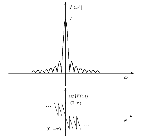
FIGURE 1.2. Top: Magnitude spectrum![]() of rectangular pulse. Notice that
of rectangular pulse. Notice that![]() has
has
zeros at![]() Bottom: Phase spectrum arg
Bottom: Phase spectrum arg![]() of rectangular pulse. Notice
of rectangular pulse. Notice
The equation for the pulse is
Let the frequency be f in Hz [cycle/s] and![]() [radian/s]. Then the
[radian/s]. Then the
Fourier transform of f (t) is
The magnitude spectrum![]() and the phase spectrum arg
and the phase spectrum arg![]() are depicted
are depicted
in Figure 1.2. Notice that arg![]() of /(f) is linear for
of /(f) is linear for![]() with jumps equal to
with jumps equal to![]() for
for![]() because of the change of sign of
because of the change of sign of![]() at these points.
at these points.
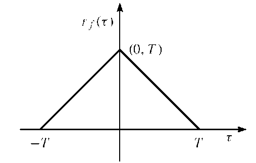
From (1.4) follows that the![]() for a rectangular pulse has a triangular waveform; see Figure 1.3,
for a rectangular pulse has a triangular waveform; see Figure 1.3,
FIGURE 1.3. Autocorrelation function![]() of the rectangular pulse shown in Figure 1.1.
of the rectangular pulse shown in Figure 1.1.
The energy density spectrum![]() of f(t) is a real function because
of f(t) is a real function because![]()
![]()
The energy density spectrum of the rectangular pulse f (t) is
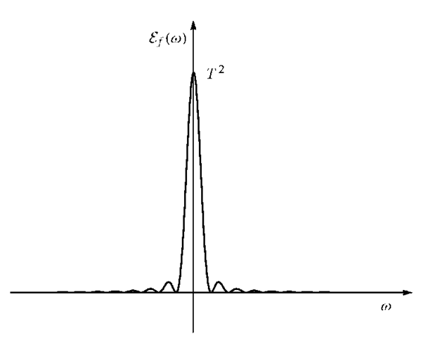
The energy density spectrum![]() is depicted in Figure 1.4. In discrete time the rectangular pulse takes on the form
is depicted in Figure 1.4. In discrete time the rectangular pulse takes on the form
where N is an integer. The Fourier transform of f (n) is
Random Signals
A random process can be viewed as a mapping of the outcomes of a random experiment to a set of functions of time—in this context a signal X (t). Such a signal is stationary if the density functions p(X (t)) describing it are invariant under translation of time t. A random stationary process is an infinite energy signal, and therefore its Fourier transform does not exist. The spectral characteristics of a random process is obtained according to the Wiener-Khinchine theorem by computing the Fourier transform of the ACF. That is, the distribution of signal power as a function of frequency is given by
FIGURE 1.4. Energy density spectrum![]() of the rectangular pulse shown in Figure 1.1. Note that
of the rectangular pulse shown in Figure 1.1. Note that![]() has zeros at
has zeros at![]()
The ACF of the stationary process X (t) is defined as![]()
with![]() denoting the expectation operator and
denoting the expectation operator and![]() being the lag. The inverse Fourier transform is given by
being the lag. The inverse Fourier transform is given by
The quantity![]() is called the power density spectrum of X (t).
is called the power density spectrum of X (t).
A discrete-time random process (sequence) has infinite energy but has a finite average power given by![]() According to the Wiener-Khinchine theorem we obtain the spectral characteristic of the discrete-time random process by means of the Fourier transform of the autocorrelation sequence
According to the Wiener-Khinchine theorem we obtain the spectral characteristic of the discrete-time random process by means of the Fourier transform of the autocorrelation sequence![]()
The inverse Fourier transform is
Random Sequence of Pulses
In Section 1.1.4 we studied the characteristics of a single rectangular pulse f (t). Next we want to become familiar with the same properties for a random sequence of pulses with amplitude ±1; each pulse with duration T.
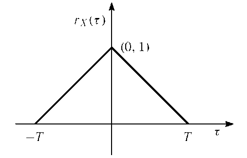
FIGURE 1.5. Autocorrelation function![]() for random sequence of pulses with amplitude
for random sequence of pulses with amplitude![]()
The ACF for the sample function x (t) of a process X (t) consisting of a random sequence of pulses with amplitude![]() and with equal probability for the outcome + 1 and —1 is
and with equal probability for the outcome + 1 and —1 is ![tmp2D170_thumb[2] tmp2D170_thumb[2]](http://what-when-how.com/wp-content/uploads/2012/02/tmp2D170_thumb2_thumb.png)
The ACF is plotted in Figure 1.5. It follows that the power spectral density is
which is plotted in Figure 1.6. The power spectral density of X (t) possesses a main lope bounded by well-defined spectral nulls. Accordingly, the null-to-null bandwidth provides a simple measure for the bandwidth of X (t).
Note that the power spectral density![]() of a random sequence of pulses with amplitude
of a random sequence of pulses with amplitude![]() differs from the energy spectral density
differs from the energy spectral density![]() given in (1.11), of a single rectangular pulse by only a scalar factor T.
given in (1.11), of a single rectangular pulse by only a scalar factor T.

![tmp2D97_thumb[2] tmp2D97_thumb[2]](http://what-when-how.com/wp-content/uploads/2012/02/tmp2D97_thumb2_thumb.png)
![tmp2D100_thumb[2] tmp2D100_thumb[2]](http://what-when-how.com/wp-content/uploads/2012/02/tmp2D100_thumb2_thumb.png)
![tmp2D117_thumb[2] tmp2D117_thumb[2]](http://what-when-how.com/wp-content/uploads/2012/02/tmp2D117_thumb2_thumb.png)

![tmp2D128_thumb[2] tmp2D128_thumb[2]](http://what-when-how.com/wp-content/uploads/2012/02/tmp2D128_thumb2_thumb.png)
![tmp2D129_thumb[2] tmp2D129_thumb[2]](http://what-when-how.com/wp-content/uploads/2012/02/tmp2D129_thumb2_thumb.png)
![tmp2D132_thumb[2] tmp2D132_thumb[2]](http://what-when-how.com/wp-content/uploads/2012/02/tmp2D132_thumb2_thumb.png)
![tmp2D134_thumb[2] tmp2D134_thumb[2]](http://what-when-how.com/wp-content/uploads/2012/02/tmp2D134_thumb2_thumb.png)
![tmp2D135_thumb[2] tmp2D135_thumb[2]](http://what-when-how.com/wp-content/uploads/2012/02/tmp2D135_thumb2_thumb.png)

![tmp2D152_thumb[2] tmp2D152_thumb[2]](http://what-when-how.com/wp-content/uploads/2012/02/tmp2D152_thumb2_thumb.png)
![tmp2D159_thumb[2] tmp2D159_thumb[2]](http://what-when-how.com/wp-content/uploads/2012/02/tmp2D159_thumb2_thumb.png)
![tmp2D160_thumb[2] tmp2D160_thumb[2]](http://what-when-how.com/wp-content/uploads/2012/02/tmp2D160_thumb2_thumb.png)

![tmp2D171_thumb[2] tmp2D171_thumb[2]](http://what-when-how.com/wp-content/uploads/2012/02/tmp2D171_thumb2_thumb.png)
