Introduction
Textural information is increasingly recognized as being useful in the classification of remotely sensed imagery. Many algorithms for the quantification of texture have been proposed, such as second-order statistics derived from the grey level cooccurrence matrix (Haralick et al., 1973) and geostatistical measures of spatial variability (Miranda et al., 1992, 1996; Ramstein and Raffy, 1989) and most are derived from a sliding window area passed over the imagery. Although combining spectral with textural information generally results in an increase in classification accuracy over that derived from a standard spectral classification, textural information has been used relatively rarely. A major reason for this situation is that there is no general rule as to which textural measures should be used and perhaps more importantly, what size of a sliding window should be chosen for their derivation. Most applications, therefore, have significant shortcomings with texture derived from a moving kernel of a fixed size, where window size is chosen experimentally in the pre-processing phase and may be appropriate for only the particular data used in a specific study.
In this topic, issues connected with the uncertainty in land cover mapping from remotely sensed data are addressed. The main focus is on evaluating the potential of a variogram-based algorithm for the quantification of image texture. Focusing on the optimal use of variogram-derived texture measures, two sets of variables were used. Firstly, a number of texture bands derived within a kernel of an adapting size (Franklin and McDermid, 1993; Franklin et al., 1996) was used in image classification. Secondly, the size of an adapting window, being a measure of both texture and border proximity, was used as an additional input to the classification. Additionally, attention was focused on areas located in the proximity of boundaries between classes which are particularly problematical in image classification, particularly when using textural measures. The research used medium spatial resolution optical (Landsat-5 TM) and microwave (ERS-1 SAR) imagery of an area characterized by a complex mosaic of small land cover patches. Due to the high density of boundaries in the study area, the size of the kernel for texture quantification was of particular importance in terms of the accuracy of the resulting classification. Finally, the uncertainty in class allocation resulting from the application of a neural network classifier to the derived data is discussed in this topic. Two criteria, the magnitude of class membership strength and the difference in memberships observed for a pixel (Gopal and Woodcock, 1994), were used to discriminate between pixels allocated to a class with a high degree of confidence, those for which an uncertain allocation was made and those for which it may be most appropriate to leave unclassified.
The variogram and its applications in image classification
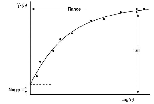
The variogram, is a function of variance with distance that describes the spatial dependence in a data set (Figure 7.1). Generally observations that are close in space are more alike than those that are far apart. In the bounded model of the variogram, semivariance reaches its maximum (sill) at a distance over which the data are correlated (range). The nugget of the variogram indicates the level of spatially independent noise present.
Figure 7.1 Variogram and its characteristic features: sill, nugget and range
The experimental variogram can be described mathematically by equation (1) (Cressie, 1993):
where n(h) is the number of pairs in lag h, dn() represents the image digital number values at location x,- and x,- + h; and k denotes a waveband.
Multivariate variograms (Journel and Huijbregts, 1978; Wackernagel, 1995) measure the joint spatial variability between two wavebands (the cross variogram) equation (2):
and the variance of cross-differences of two wavebands (the pseudo-cross variogram) equation (3):
where j and k indicate two radiometric wavebands (e.g. spectral wavebands or, as in this study, two principal components images derived from the remotely sensed data).
Geostatistics, and the variogram in particular, are currently well understood and frequently applied in image analysis. It has been shown (Woodcock et al., 1988a, 1988b) that the variogram’s range is directly related to texture and/or object size, while its sill is proportional to the global object (class) variance, although it is also affected by external factors, such as sensor gain, image noise, atmospheric conditions etc.
Recently there has been increasing interest in the potential applications of vario-gram-derived texture measures for use in image classification. Two approaches to the derivation of texture from the variogram have been suggested and used to increase image classification accuracy: the semivariogram textural classifier algorithm (STC, Miranda et al., 1992, 1996) and methods based on the coefficients of the variogram model (Ramstein and Raffy, 1989). In STC, semivariances for the first consecutive lags are used directly as additional input layers to an image classification, while in the second technique, variogram model coefficients are used. However, the general application of both techniques has an important shortcoming in that the computation of the variogram is typically based on a moving window area or kernel of a fixed size.
There is a trade-off between the application of a window that is too large, and one that is too small. The first approach leads to the window straddling class boundaries, and so encompassing different classes in adjacent areas in the same variogram. On the other hand, the sill of a variogram may be not achieved if the calculations are undertaken within a small window. Furthermore, variograms for short lags measure field edges rather than within-field variability that is important texturally (Jako-mulska and Stawiecka, 2002). Franklin and McDermid (1993) and Franklin et al. (1996) proposed an alternative technique, a geographic window in which the dimensions of a moving kernel are customized and are determined by the variogram’s range. The range of a variogram is short for homogeneous objects (e.g. water) and increases for more textured objects. Furthermore, the range contracts at object boundaries while the variance increases very rapidly due to the fact that the window straddles the boundary separating adjacent areas of different classes. These features allow the moving window to remain small when the edge of an object is approached. The geographic window based technique has proved to be promising in the derivation of textural measures (Wulder et al., 1997).
Unfortunately, no consensus has been reached on which textural measures are appropriate to achieve the greatest accuracy in image classification. Although Ram-stein and Raffy (1989) showed that some land cover classes can be well differentiated using only the range of the variogram (assuming an exponential variogram model), other reports show that both the sill and range are distinctive for different land cover types (St-Onge and Cavayas, 1995; Wallace et al., 2000; Jakomulska and Clarke, 2001). The range of variogram indicates the coarseness of texture and has been shown to be an important discriminant of a variety of land cover classes. However, the variogram’s range is also directly related to the size of objects (and boundary proximity): for small patches (in landscapes characterized by high spatial frequency) the range of a variogram is shorter than for large patches. Hence, it seems inappropriate to use a constant value.
Increases in classification accuracy through the use of textural information have also generally been observed in studies with relatively ideal conditions. For example, studies have used fine spatial resolution data in which the high variance of objects results from the amount of detail present in the image (Wharton, 1982; Wulder et al., 1996, 1998), microwave imagery in which the textural analysis reduces speckle noise and works like a low pass filter (Miranda et al., 1992, 1996), and per-field image classification in which the problematical boundaries are removed (Berberoglu et al., 2000).
In this study, variogram-based measures (sills, ranges, mean semivariances, sum of semivariances up to a range and semivariances at lag = 0) were derived from a kernel of an adapting size, as proposed by Franklin and McDermid (1993). To analyse the ‘border effect’ of spatial classification, the accuracy of classification based on textural information derived from a moving window was assessed. Later also the range (the window size itself) was used as an additional textural measure. Due to the non-Gaussian distribution of textural data an artificial neural network classifier, which does not make assumptions about the data’s distribution was used.To gain an understanding of utility and limitations of the approach, attention focuses on the overall accuracy of the classification as well as the spatial distribution of error.
Study Area and Data
The study area was the Kolno Upland, located in north-eastern Poland (between 21°70′ and 22°60′E and 53°20′ and 53°60′N). The landscape was agricultural, with arable lands prevailing on the upland and meadows along valley floors. The arable lands were characterized by a complicated pattern of ownership that resulted in a mosaic of small parcels (on average 5 ha). Coniferous and deciduous forests covered a few per cent of the area. Along the valley bottoms, sparsely timbered deciduous forests were common. Urbanized areas were rare, but dispersed households and small settlements were frequent in the region.
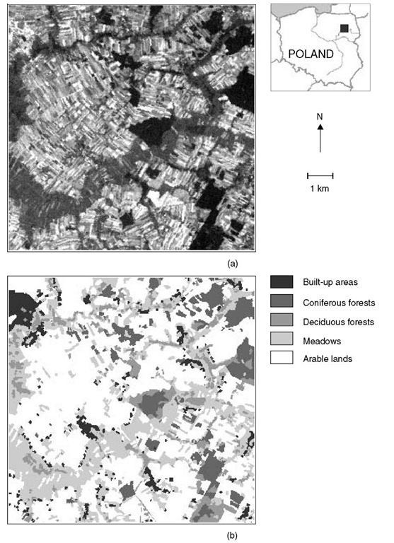
A Landsat-5 Thematic Mapper (TM) image acquired on 25 August 1987 (Figure 7.2; see also plate 1) and an ERS-1 SAR image acquired on 31 August 1994 were used. Colour aerial images at a 1:26 000 scale, acquired on 23 August 1995, were used to guide the training and accuracy assessment stages of the classification. Due to a lack of data in the same time-frame, the available data were used in spite of the large time gap between the image acquisitions. However, this approach is believed to be justifiable for two main reasons. Firstly, due to the low agricultural productivity and relative economic stagnation of the region, no major changes in land use and land ownership had occurred in the area. The main differences that occurred in the time between image acquisitions were differences in the crop mosaic which were unimportant as it was not intended to identify individual crops, but simply arable lands. Secondly, since all images were acquired at the end of August, after harvest, the arable lands consisted of exposed bare soils with a varied tillage pattern. The following land cover classes were therefore analysed: built-up areas, coniferous forests, deciduous forests, meadows and arable lands.
Pre-processing of the data was limited to geometric and radiometric correction of the data. Speckle noise removal was a necessary pre-processing step in the analysis of the microwave imagery to reduce the random variation present. To reduce the speckle present in the SAR image, a Gamma-Map (Maximum a Posteriori) filter (3 x 3 window) was applied to it (Frost et al., 1982). The filter is based on a multiplicative noise model with non-stationary mean and variance and assumes Gamma distribution for the speckle noise. The ERS-1 SAR image was resampled to the pixel size of Landsat TM and compressed to 8-bit radiometric resolution (using a two standard deviations stretch). Similarly, ground data, acquired through photo-interpretation were converted to a raster format and resampled to the spatial resolution of the non-thermal Landsat TM data. All of the image data were georeferenced to a standard reference system using nearest neighbour resampling and a second-order transformation equation (RMSE = 0.34 for Landsat TM and RMSE = 0.47 for ERS-1 SAR data).
The pre-processing of the Landsat TM image did not influence the textural information content of the data (since nearest neighbour resampling was employed). On the other hand, the ERS-1 SAR data, were subjected to three pre-processing processes (filtering, resampling, rescaling), which, although necessary, might degrade the data’s textural information content (via smoothing).
Spectral and textural characteristics of the studied land cover classes
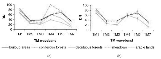
The Landsat TM sensor was specifically designed for studies such as land cover mapping. However, in spite of a small number of classes analysed in this study, the land cover classes do not exhibit perfect separability (Figure 7.3). The within-class variance was typically very large, with considerable overlap of the ranges of the observed spectral responses, particularly for the built-up areas and arable lands classes. The large within-class variance of the built-up class resulted from the varied land cover found within this class. Arable lands were highly varied due to the complex mosaic of small land parcels found at the site.
Figure7.2 Testsite. (a) Central part of Kolno Upland: red band of LandsatTM. (b) Ground data achieved through visual interpretation of aerial images.
Figure 7.3 Spectral separability of the classes. (a) Spectral responses. (b) Within-class variation for three classes. Vertical bars mark standard deviation
Spatial information is of particular benefit for mapping classes characterized by large within-class variance (even if the within-class variance is larger than the inter-class variance). For example, variograms derived from training samples show that built-up areas can be easily distinguished from arable lands using sills of variograms derived from the red waveband (Figure 7.4).


