Introduction
Remote sensors, whether carried by aircraft or satellites, are widely used to provide synoptic information about large areas of the Earth’s surface. As an information source, they are particularly attractive because they can acquire data for a large ground area almost instantaneously, regardless of geographic accessibility. The information they acquire has a wide range of applications within industry, government and academia, including guiding prospectors to important sources of natural resources, measuring crop acreage to allow quotas to be efficiently enforced, and monitoring rates of deforestation.
Remote sensing is a complex process in which, generally, electromagnetic radiation emitted by the Sun is reflected by objects on the ground, travels through the atmosphere, and, in the case of satellite-based sensors, through space, before arriving at the sensor. In the sensor, some physical change is caused, which is typically measured electronically and stored digitally before being transmitted back to Earth. There are thus many stages between the radiation leaving the Sun, and information about the sensor measurement reaching its final application within which uncertainty about the actual reflective properties of the ground cover can be introduced.
The overwhelming complexity of the remote sensing process has so far frustrated all attempts to produce comprehensive physical models of the uncertainty present in remotely sensed data. The first part of the research presented in this topic attempts to increase the understanding of this uncertainty by examining the effect of one source of ambiguity – the transfer function of the sensor itself – within one domain – estimating the areas of different land cover classes. From this starting point, the uncertainty introduced by the sensor can be characterized in some detail, and the results generalized to other applications.
Despite the advances that will be discussed, a full analytical characterization of the uncertainty in remotely sensed data (and quantities derived from it) is still not possible, and perhaps never will be. The second section of this topic, therefore, focuses on a statistical technique that is capable of learning, by example, the exact form of the ambiguity present in quantities derived from remotely sensed data, thus avoiding the need to develop complex analytical models altogether. To demonstrate how the technique should be applied in practice, and what information it can be expected to produce, it was applied to a real-world, area estimation, problem.
A Theoretical Analysis of the Ambiguity Induced by the PSF
One of the great challenges in developing models of the uncertainty present in remotely sensed data, and, perhaps more importantly, information derived from them, is to make statements that are sufficiently general. For example, it is sometimes possible to gain insights into the sources of uncertainty in specific remote sensing activities that have occurred in the past. Unless these insights can be generalized to future activities, however, they are of little use.
One way to guarantee that research is of the broadest relevance is to examine some aspect of the remote sensing process that is common to a large proportion of applications. Perhaps the most obvious (but least studied) of these are to do with the characteristics of the sensor itself. Results pertaining to a particular type of sensor are likely to apply to every situation in which the sensor is used, and as the research in this topic will show, the sensor is an important source of uncertainty, which places a fundamental limit on the amount of information that remotely sensed data can contain.
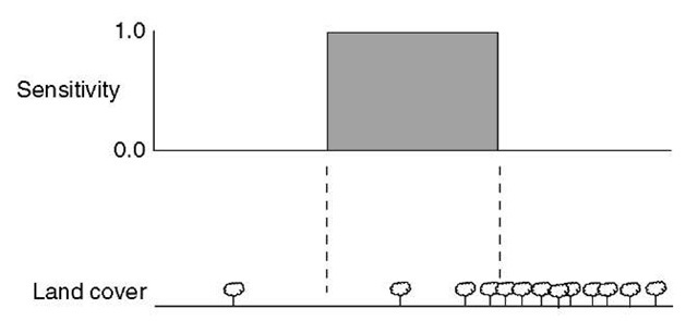
Traditionally, the output of a remote sensor is represented as a series of raster images, each containing information on the reflectance of the target area in one of the spectral bands in which the sensor operates (Fisher, 1997). These images consist of regular grids of rectangular pixels, and each pixel is usually considered to correspond to some well-defined area of the ground beneath the sensor, as shown for a single row of pixels in Figure 4.1. The reflectance information given by each pixel is assumed to be the average of the reflectance of the land cover within the corresponding area of the ground, and unaffected by the reflectance of land cover outside it, as shown for a single pixel in one row of an image in Figure 4.1.
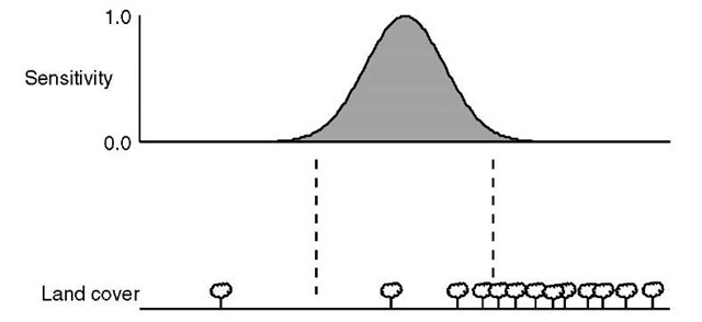
In practice, the characteristics of remote sensors are far from ideal (Cracknell, 1998). One of their deficiencies is that the reflectance information contained within a single pixel is affected by land cover outside the area of ground normally associated with it. This can be seen by comparing Figures 4.1 and 4.2. In the former, the sensitivity of the ideal sensor is, for a single pixel, zero outside the area of ground that is associated with it, whereas the sensitivity of the real sensor is non-zero into the area covered by neighbouring pixels. This inter-pixel interference effect is discussed in greater detail in Townshend et al. (2000), where a method of compensating for it is described.
Figure 4.1 An idealized sensor is uniformly sensitive to the reflectance of all land cover within the pixel area (which lies between the dashed lines). Outside this area, the sensor has zero sensitivity and is unaffected by the reflectance of the land cover there.
Figure 4.2 In practice, the sensitivity of real sensors varies within the pixel area (which lies between the dashed lines). Outside the pixel, the sensor has non-zero sensitivity and hence the reflectance measured for a pixel is affected by land cover that lies outside it.
Another undesirable characteristic of real sensors is shown in Figure 4.2, where the sensor is not uniformly responsive to the reflectance of land cover within the area of ground associated with each pixel (Justice et al., 1989). Most sensors exhibit sensitivity variation similar to that shown in Figure 4.2 – being most sensitive to land cover in the centre of a pixel’s ground area, and least sensitive towards its edge. The reflectance information contained in a pixel thus tends to be most similar to the reflectance of land cover located towards the centre of the pixel’s ground area, and least similar to cover towards its edge. This variation in sensitivity is described by a function, called the point spread function (PSF) of the sensor, and its practical effects – which have, until fairly recently, been largely ignored – are considered in this topic.
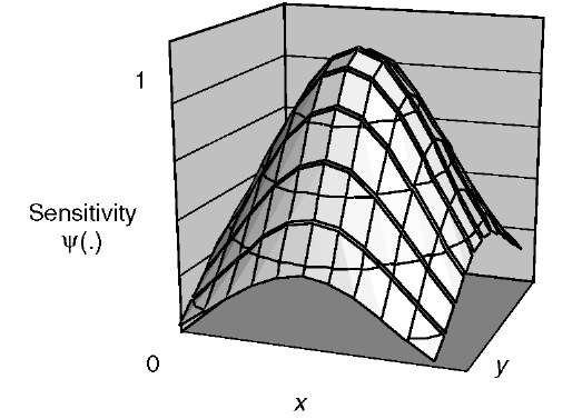
Since a pixel has a two-dimensional ‘footprint’ on the ground, a real PSF has a shape similar to that shown in Figure 4.3. The horizontal axes correspond to the distance on the ground of a point from the centre of the area that a pixel covers on the ground, and for each point, the height of the function gives the sensitivity of the sensor relative to its maximum sensitivity. The PSF shown is Gaussian – that is, if r is the distance of a point (x,y) on the ground from the point of maximum sensitivity, the sensor’s sensitivity![]() is given by:
is given by:
Figure 4.3 A Gaussian model of a PSF with parameter a = 2. The dark grey square at the figure’s base represents the ground area that the pixel would normally be considered to cover. The ‘height’ of the surface above a point on this square indicates the sensitivity of the remote sensor to the reflectance of ground cover at that point compared to that at the pixel’s centre. For example, the sensitivity of the sensor to land cover located at the nearest corner of the pixel is less than one-fifth that at its centre.
where a controls how quickly the sensitivity falls off as the distance from the point of maximum sensitivity increases. Although this PSF model is simplistic (for example, real PSFs do not usually possess exact circular symmetry), it is easy to analyse mathematically.
In order to make the present discussion of the effect of a sensor’s PSF more concrete, it will be considered in the context of the problem of estimating the areas of land cover classes from remotely sensed imagery. This does not limit the generality of the results that are derived, however, since they relate fundamentally to the ambiguity that a sensor’s PSF creates regarding all processes that occur at ground level. Estimates of the areal extent of land cover classes have been extracted from remotely sensed images for a long time. This has generally been achieved by classifying each pixel in an image into one of a predefined set of classes. Since the area covered by the image is usually known, counting the number of pixels belonging to each class yields an estimate of their areas.
This area estimation by pixel classification process produces area estimates with rather large errors – typically too large to be useful in most applications. One of the more promising developments that aimed to reduce the magnitudes of these errors recognized that the area of ground covered by a particular pixel may not be homogeneous – that is, there may be several different cover types within it. This critical realization led to the development of sub-pixel proportion estimation algorithms that attempt to estimate the proportion of the sub-pixel area covered by each of the classes of interest,and can be considered to be the current state of the art.
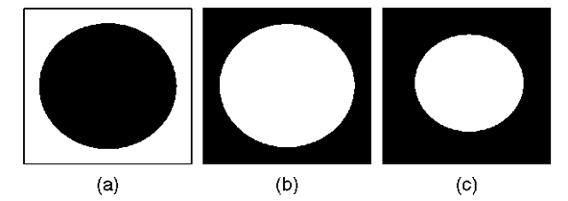
In Manslow and Nixon (2000) it was shown that sensitivity variation within the PSF of a sensor introduces ambiguity into these proportion estimates. To illustrate this, Figure 4.4 shows an abstract plan-view representation of the area of ground covered by three pixels.
Figure 4.4 Representations of the sub-pixel arrangement of land cover for three pixels. Each of the three squares represents a plan view of the ground area associated with one of three pixels in a remotely sensed image. The pixel areas are divided between two classes, represented in black and white. Pixel (a) contains the two classes in equal proportions, and the black class is arranged in the centre, and the white class towards its perimeter. Pixel (b) is identical to pixel (a) except that the locations of the classes are swapped. Pixel (c) is identical to pixel (b), except that the area of the black class has been increased so that the remote sensor observes the same reflectance as for pixel (a)
In the first pixel, Figure 4.4(a), the sub-pixel area is divided equally between two classes, one located centrally (shown in black), and the other located towards the pixel’s perimeter (shown in white). Since most PSFs display greatest sensitivity to the reflectance of land cover that is located centrally (as shown in Figure 4.3), the measured reflectance of the pixel will be most similar to the centrally located class – the black class.
The second pixel, shown in Figure 4.4(b), is identical to the first, except that the classes have been swapped over – the black class now lies towards the pixel’s perimeter, and the white class, at its centre. Once again, because the PSF gives the sensor greatest sensitivity to centrally located land cover, the reflectance that is measured will be most similar to that of the centrally located class – in this case, the white class. Although the proportions with which the black and white classes are present in the pixels in Figures 4.4(a) and 4.4(b) are identical, a different reflectance is measured in each case.
Now consider taking the pixel in Figure 4.4(b), and gradually increasing the proportion of the black class, as shown in Figure 4.4(c). As more and more of the black class is added, the reflectance of the pixel would increasingly come to resemble that of the black class until, eventually, the pixel had the same reflectance as that in Figure 4.4(a). Thus, although a remote sensor would measure identical reflectances for the pixels in Figures 4.4(a) and 4.4(c), their sub-pixel compositions are distinct not simply in terms of the spatial arrangement of the sub-pixel cover, but also in terms of the proportions in which the classes are present. This indicates that a pixel’s reflectance contains only ambiguous information about its composition.
The above effect was analysed in more detail by Manslow and Nixon (2000) using the Gaussian PSF model that was introduced earlier. Making use of the simplifying assumptions that a pixel has a circular footprint, area n, and that there are only two sub-pixel classes, which exhibit no spectral variation, it was possible to derive upper bounds on the ambiguity induced by the PSF. In particular, assuming a pixel has been observed, which contains two sub-pixel classes, which cover areas ai and a2, pixels with identical reflectances may also exist where the first class covers an area anywhere from
to
where
and
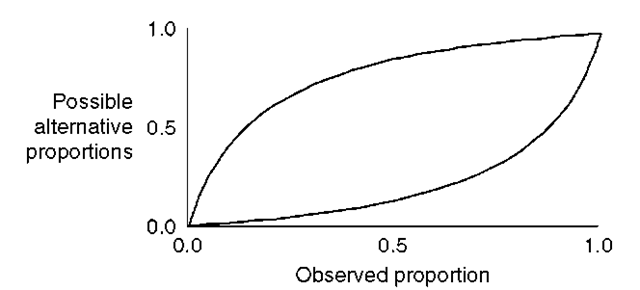
These limits can be interpreted as upper bounds on the ambiguity induced by the Gaussian PSF because they define the range over which sub-pixel proportions can vary without any change in a pixel’s measured reflectance. The bounds are plotted in Figure 4.5 and have a number of interesting properties:
1. The amount of ambiguity can be expressed as a function of the degree of sub-pixel mixing, making it easy to assess the impact of the PSF on sub-pixel area estimates.
2. The amount of ambiguity is not dependent on the level of spectral separation of the classes. The effect of the PSF is the same regardless of whether the classes are spectrally very similar, or highly distinct.
3. The amount of ambiguity induced by the PSF increases with the amount of sub-pixel mixing. That is, greatest ambiguity is induced when the sub-pixel area is partitioned equally between the two classes.
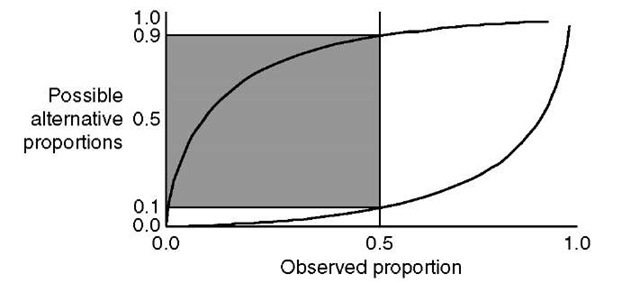
Figure 4.6 provides a simple illustration of how to interpret the bounds for a pixel that contains two sub-pixel classes present in equal proportions. To find the bounds on the ambiguity induced by the PSF, a line is drawn up from the x-axis from the point x = 0.5 (indicating that one of the classes covers 50% of the sub-pixel area).
Figure 4.5 The bounds on the ambiguity induced by a Gaussian PSF with a = 2 calculated analytically, as in this figure, are almost identical to those predicted by the computational technique. This suggests that the grid-based approximations used in the latter have minimal impact on the accuracy of the predicted bounds. Note how the bounds are widest when one of the sub-pixel classes covers a proportion of around 0.5 of the sub-pixel area.
Figure 4.6 Ambiguity induced by the Gaussian PSF with a = 2 calculated by the computational technique. When a proportion of 0.5 of sub-pixel area is known to be covered by a class, other pixels could also exist, that cannot be distinguished by a remote sensor, where the same class covers anywhere between a proportion of 0.1 and 0.9 of the sub-pixel area.
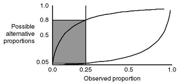
The y-coordinate of the point where the line intersects the lower curve – in this case about 0.1 – gives the minimum proportion that the class could cover in other pixels with the same spectral properties as the one currently being considered. Similarly, the y-coordinate of the point where the line intersects the upper curve – in this case, around 0.9 – gives the maximum proportion that the class could cover. Thus, for the Gaussian model of the PSF that was described earlier, if a pixel is known to contain two classes in equal proportions, other pixels may also exist, which are spectrally identical, but where either of the classes cover anywhere between 10 to 90% of the sub-pixel area. Since the pixels are spectrally identical, they cannot be distinguished by a remote sensor, regardless of how spectrally distinct the individual classes are. Figure 4.7 shows another example where the same process has been applied to estimate the bounds when a pixel is known to be divided between two classes in the proportions 0.25 to 0.75. In this case, other, spectrally identical pixels exist where the first class covers anywhere between 5 and 80% of the sub-pixel area.
Before pursuing the implications of the above discussion further, it is important to consider how, and indeed whether, they can be extended to more realistic PSF models. Although the analytical examination of a Gaussian model of a PSF (presented in detail in Manslow and Nixon, 2000) produces important insights, it cannot easily be extended to other PSF models because of the intractability of the analysis that is required.
Figure 4.7 Ambiguity induced by the Gaussian PSF with a = 2 calculated by the computational technique. When a proportion of 0.25 of sub-pixel area is known to be covered by a class, other pixels could also exist, that cannot be distinguished by a remote sensor, where the same class covers anywhere between a proportion of 0.05 and 0.8 of the sub-pixel area.
The following section describes an efficient computational technique for deriving bounds on PSF-induced ambiguity that can be applied to almost any PSF model to arbitrary accuracy, provided that sufficient computing power is available.
