Jaccard coefficient:
A similarity coefficient for use with data consisting of a series of binary variables that is often used in cluster analysis. The coefficient is given by
where a, b and c are three of the frequencies in the 2 x 2 cross-classification of the variable values for subjects i and j. The critical feature of this coefficient is that ‘negative matches’ are excluded.for reducing bias in estimation and providing approximate confidence intervals in cases where these are difficult to obtain in the usual way. The principle behind the method is to omit each sample member in turn from the data thereby generating n separate samples each of size n — 1. The parameter of interest, 0, can now be estimated from each of these subsamples giving a series of estimates, 0^,02,… ,0n. The jackknife estimator of the parameter is now
where 0 is the usual estimator using the complete set of n observations. The jackknife estimator of the standard error of 0 is
where
A frequently used application is in discriminant analysis, for the estimation of misclassification rates. Calculated on the sample from which the classification rule is derived, these are known to be optimistic. A jackknifed estimate obtained from calculating the discriminant function n times on the original observations, each time with one of the values removed, is usually a far more realistic measure of the performance of the derived classification rule.
Jacobian leverage:
An attempt to extend the concept of leverage in regression to non-linear models, of the form
where fi is a known function of the vector of parameters h. Formally the Jacobian leverage, jik is the limit as b ! 0 of
where 9 is the least squares estimate of 9 and 9(k, b) is the corresponding estimate when yk is replaced by yk + b. Collecting the jik s in an n x n matrix J gives
where e is the n x 1 vector of residuals with elements e,- = y,- — f- (9) and [e'][W] = J]n= 1 eWW,- denotes the Hessian matrix of f-(9) and V is the matrix whose ith row is @fi(9)/99′ evaluated at 9 = 9. The elements of J can exhibit super-leverage.
James-Stein estimators:
A class of estimators that arise from discovery of the remarkable fact that in a multivariate normal distribution with dimension at least three, the vector of sample means, x, may be an inadmissable estimator of the vector of population means, i.e. there are other estimators whose risk functions are everywhere smaller than the risk of x, where the risk function of an estimator is defined in terms of variance plus bias squared. If X’ = [X1, X2,..., Xp] then the estimators in this class are given by
If a is sufficiently small and b is sufficiently large, then Sa’b has everywhere smaller risk than X.
Jeffreys, Sir Harold (1891-1989):
Born in Fatfield, Tyne and Wear, Jeffreys studied at St John’s College, Cambridge where he was elected to a Fellowship in 1914, an appointment he held without a break until his death. From 1946 to 1958 he was Plumian Professor of Astronomy. Made significant contributions to both geophysics and statistics. His major work Theory of Probability is still in print nearly 70 years after its first publication. Jeffreys was made a Fellow of the Royal Society in 1925 and knighted in 1953. He died in Cambridge on 18 March 1989.
Jeffreys’s prior:
A probability distribution proportional to the square root of the Fisher information.
Jelinski-Moranda model:
A model of software reliability that assumes that failures occur according to a Poisson process with a rate decreasing as more faults are discovered. In particular if 0 is the true failure rate per fault and N is the number of faults initially present, then the failure rate for the ith fault (after i — 1 faults have already been detected, not introducing new faults in doing so) is
Jenkins, Gwilym Meirion (1933-1982): Jenkins obtained a first class honours degree in mathematics from University College, London in 1953 and a Ph.D. in 1956. He worked for two years as a junior fellow at the Royal Aircraft Establishment gaining invaluable experience of the spectral analysis of time series. Later he become lecturer and then reader at Imperial College London where he continued to make important contributions to the analysis of time series. Jenkins died on 10 July 1982.
Jensen’s inequality:
For a discrete random variable for which only a finite number of points y1; y2;…; yn have positive probabilities, the inequality
where = E(y) and g is a concave function. Used in information theory to find bounds or performance indicators.
Jewell’s estimator:
An estimator of the odds ratio given by
where a, b, c and d are the cell frequencies in the two-by-two contingency table of interest. See also Haldane’s estimator.
Jittered sampling:
A term sometimes used in the analysis of time series to denote the sampling of a continuous series where the intervals between points of observation are the values of a random variable.
Jittering:
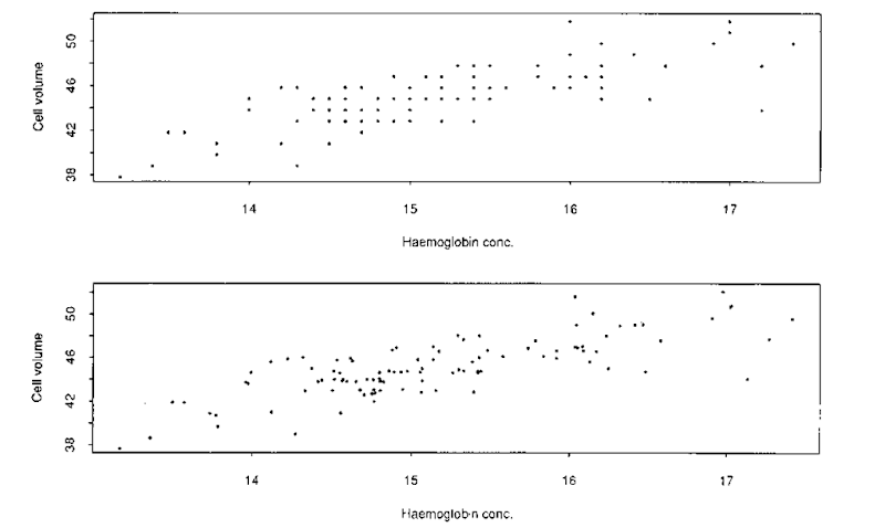
A procedure for clarifying scatter diagrams when there is a multiplicity of points at many of the plotting locations, by adding a small amount of random variation to the data before graphing. An example is shown in Fig. 77.
Johnson’s system of distributions:
A flexible family of probability distributions that can be used to summarize a set of data by means of a mathematical function which will fit the data and allow the estimation of percentiles. Based on the following transformation
where y is a standard normal variable and the k{(x, X, e) are chosen to cover a wide range of possible shapes. The following are most commonly used:
the Sv distribution;
Fig. 77 An example of ‘jittering’: first scatterplot shows raw data; second scatterplot shows data after being jittered.
the SB distribution;
the SL distribution. The SL is in essence a three-parameter lognormal distribution since the parameter k can be eliminated by setting y* = y — ^ ln k so that z = y* + ^ ln(x — 6). The SB is a distribution bounded on (e, e + k) and the Sv is an unbounded distribution.
Joint distribution:
Essentially synonymous with multivariate distribution, although used particularly as an alternative to bivariate distribution when two variables are involved.
Jolly-Seber model:
A model used in capture-recapture sampling which allows for capture probabilities and survival probabilities to vary among sampling occasions, but assumes these probabilities are homogeneous among individuals within a sampling occasion.
Jonckheere, Aimable Robert (1920-2005):
Born in Lille in the north of France, Jonckheere was educated in England from the age of seven. On leaving Edmonton County School he became apprenticed to a firm of actuaries. As a pacifist, Jonckheere was forced to spend the years of World War II as a farmworker in Jersey, and it was not until the end of hostilities that he was able to enter University College London, where he studied psychology. But Jonckheere also gained a deep understanding of statistics and acted as statistical collaborator to both Hans Eysenck and Cyril Burt. He developed a new statistical test for detecting trends in categorical data and collaborated with Jean Piaget and Benoit Mandelbrot on how children acquire concepts of probability. Jonckheere died in London on 24 September 2005.
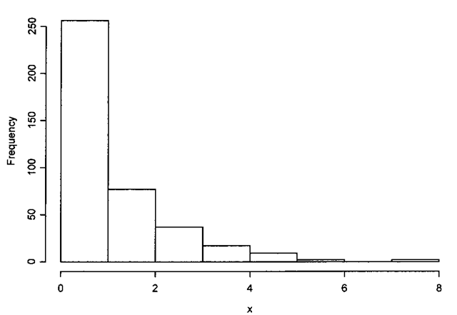
Fig. 78 An example of a J-shaped frequency distribution.
Jonckheere’s k-sample test:
A distribution free method for testing the equality of a set of location parameters against an ordered alternative hypothesis. [Nonparametrics: Statistical Methods Based on Ranks, 1975, E.L. Lehmann, Holden-Day, San Francisco.]
Jonckheere-Terpstra test:
A test for detecting specific types of departures from independence in a contingency table in which both the row and column categories have a natural order (a doubly ordered contingency table). For example, suppose the r rows represent r distinct drug therapies at progressively increasing drug doses and the c columns represent c ordered responses. Interest in this case might centre on detecting a departure from independence in which drugs administered at larger doses are more responsive than drugs administered at smaller ones.
J-shaped distribution:
An extremely asymmetrical distribution with its maximum frequency in the initial (or final) class and a declining or increasing frequency elsewhere. An example is given in Fig. 78.


