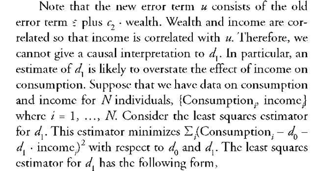
This entry explains when a variable is a predetermined variable and how identification and inference require a variable to be predetermined. In social science, researchers often try to explain a phenomenon or an event using one or more explanatory variables. For example, how much an individual earns can be explained (to some degree) by his or her education level, and how much an individual consumes can be explained by his or her income and wealth. In many cases, a social scientist will formulate a model in which one variable is a function of another variable. For example, the following is a model that relates consumption to income and wealth:
increase by $cj (that is, consumption increases by seventy cents if income increases by one dollar). In order to estimate this model, we need to extend the model with an error term. This error term captures variables other than income or wealth. Let
with income and wealth, then income and wealth are exogenous variables. No correlation means that we cannot use the regressors to predict the error term, that is, E(eIincome, wealth) = 0. If all the explanatory variables are exogenous variables, then the coefficients can be given a causal interpretation. Suppose that a social science researcher does not have access to data on wealth and, therefore, estimates the model
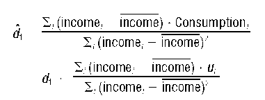
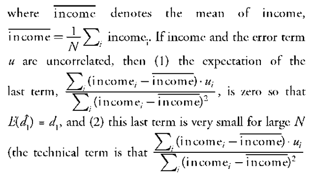
converges in probability to zero so that is a consistent estimator for dj). However, in this example, the error term u. depends on wealth. Wealth and income are correlated so that the assumption exogeneity (i.e., that all regressors are uncorrelated with the error term) is violated. As a result, the estimate for dj cannot be given a causal interpretation. In particular, the expectation of the estimator, E¥j, will be larger than 0.7 because of the positive correlation between income and wealth.
The exogeneity assumption is very strong and can be relaxed somewhat. Consider the following model that describes the squared daily return of a stockmarket (e.g., the daily return of the Standard & Poor’s 500 index),
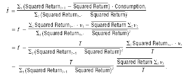
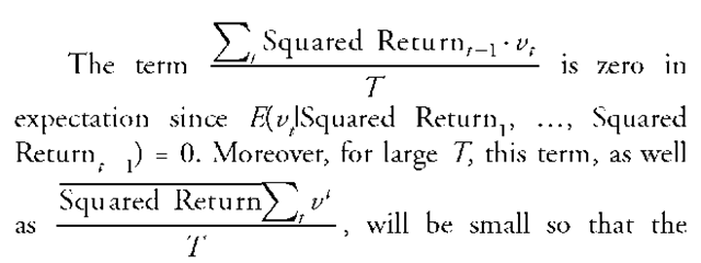
T. Rather than assuming that the correlation between the squared return and the error term is zero, that is, that E(vJSquared Return^ …, Squared Return^) = 0 for all t, we now make the weaker assumption that, given the past values of the squared return, the expectation of the error term is zero, that is, E(vJSquared Return^ …, Squared Return^_ j) = 0 for all t. Note that the past values of the squared return for error term vf consist of the squared return of the first period, Squared Returnj, through period t — 1, Squared Return t_ j. Regressors that have the property that the error term has zero expectation given past values of the regressor are called predetermined regressors or predetermined variables. Consider the least squares regressor again to see how predeterminedness helps the estimator,
estimate f is close to the true value fj. This model of squared returns is an ARCH (auto regressive conditional heteroscedasticity) model and can be used to study volatility. In particular, a large decline of the stockmarket in period t — 1 means that the stockmarket will be more volatile in period t. Tim Bollerslev, Robert Engle, and Daniel Nelson (1994) discuss other ARCH models.
An endogenous regressor has the property that E(vtISquared Returnj, …, Squared Returnt_ j) ^ 0. Thus, an endogenous regressor cannot be a predetermined regressor. Endogeneity (i.e., having an endogenous regressor) occurs if there is a third unobserved variable that affects both the regressor and the error term. For example, how much an individual earns can be partly explained by his or her education. Data on earnings and education levels are not hard to collect, but reliable data on intelligence are difficult to obtain. For this reason, earnings are usually regressed on the education so that intelligence is part of the error term. However, intelligence will also affect education levels so that the regressor education and the error term are correlated. In other words, there is an unobserved variable that affects both the regressor and the error term so that E(vJSquared Return^ …, Squared Return t_ j) ^ 0. Therefore, least squares cannot be used to estimate the effect of education on income. Econometricians have developed another technique, namely, two-stage least squares.
In nonlinear models, a slightly different definition of exogeneity and predeterminedness is sometimes used. In particular, the regressors are exogenous if the regressors and the error term are statistically independently distributed. That is, if the density of the error term conditional on the regressors, p(error termlregressors) is the same as the unconditional density of the error term, p(error term). Similarly, the regressors are predetermined if the density of the error term of period t conditional on the past regressors, p(error termjregressors^ …, regressort_ j), is the same as the unconditional density of the error term, p(error term^ for all t. Robert De Jong and Tiemen Woutersen (2006) use these definitions when they estimate a model to predict monetary policy.


