Both the method of moments and its generalization, namely the generalized method of moments (GMM), have taken a prominent place in statistical inference in the social sciences and have been applied in almost every field of economics, including asset pricing, business cycle, commodity market, education, and labor market. The (standard) method of moments consists of estimating a parameter [ by equating sample moments with population moments and solving these equations for [. This method was introduced at the end of the nineteenth century by the British mathematician Karl Pearson and was partly abandoned when the British biologist Ronald Fisher (1890-1962) showed that the maximum likelihood estimator (MLE) is more efficient than the method of moments estimator because its variance is smaller. Since its introduction by Lars Peter Hansen in 1982, however, GMM has been extremely popular in economics for three reasons. The first reason is that economic models are often too complex to be completely specified and an attempt to describe the full model is likely to yield misspecification errors. GMM provides a way to estimate partially specified models. The second reason is that, even if the model is completely specified, MLE may be too cumbersome to implement, whereas GMM provides a practical method to perform inference. Finally, GMM embeds many familiar estimation techniques as special cases, including the method of moments, ordinary least squares, instrumental variables estimation, and even maximum likelihood estimation.
THE ESTIMATION METHOD
GMM may be illustrated in a time series context where
population mean needs to be replaced by the sample mean
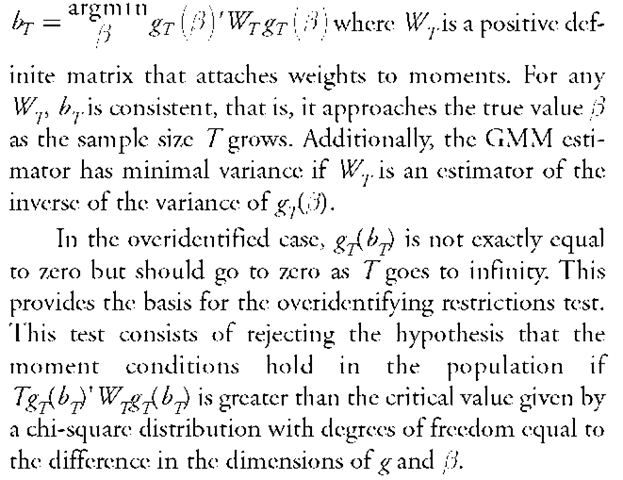
Two cases are distinguished, depending on whether the dimension of g is the same as or larger than the dimension of [ . In the first case (just identified), the equation g^ft) = 0 can be solved to obtain the method of moments estimator of ft. In the second case (overidentified), the previous equation does not have a solution and the standard method of moments needs to be modified. The GMM estimator is defined as the solution
GMM provides a framework that encompasses most estimation techniques used in economics. Instrumental variables estimation, although a predecessor to GMM, can be recast as a special case of GMM. Consider the regression
where xf is endogenous, that is, correlated with the residual £. As a consequence of endogeneity, the ordinary least squares estimator is not consistent. A consistent estimator, however, may be obtained by using a vector of so-called instruments z. To be a valid instrument, zf must be correlated with x but not with the error £.. Then, ft can be esti-
resulting estimator is called the instrumental variables estimator.
MLE itself can be interpreted as a GMM estimator because the expectation of the derivative of the log-likelihood is equal to zero, giving rise to a moment condition.
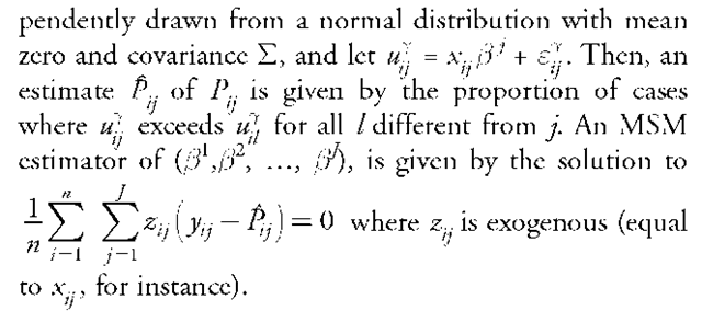
To overcome computational difficulties, Daniel McFadden (1989) and Ariel Pakes and David Pollard (1989) have proposed the method of simulated moments (MSM), which consists of replacing population moments with moments computed from simulated data.
MIXED POPULATION EXAMPLE
Consider a population where each subject is equally likely to be a male or a female. We observe a measure x (for instance, the weight) but not the sex and we wish to estimate the difference between males and females. This is particularly relevant in anthropology where most fossil specimens lack indicators of sex. Assume that observations are normally independently distributed with mean fip and variance a2 if the subject is a female and with mean fxM and the same variance a2 if the subject is a male. The method of moments that matches the expectations of x,x , and x4 with their sample counterparts permits to estimate
CONSUMPTION-BASED ASSET PRICING MODEL
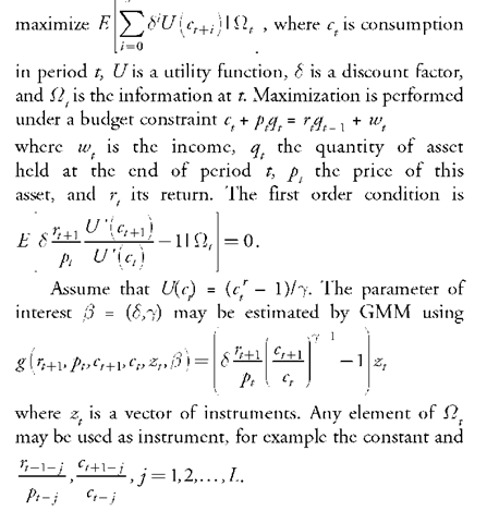
Lars Peter Hansen and Kenneth Singleton (1982) explain how to apply GMM to estimate behavioral parameters of economic agents in a general equilibrium model, without having to describe the full economic environment. This approach may be used to study how agents allocate their spending. Consider an economy where a representative agent chooses consumption and investment plans so as to
DISCRETE CHOICE MODEL
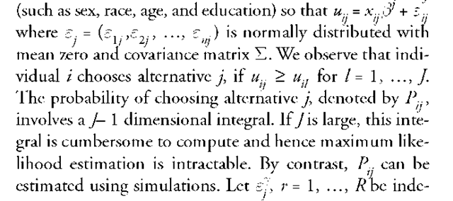
Consider a model where each individual has the choice among J alternatives (for example, occupations or means of transportation). The individual chooses the alternative with the greatest value. The value u.. of occupation j for individual i depends on a set of observed variables x..


