Ordinary least squares (OLS) is a method for fitting lines or curves to observed data in situations where one variable (the response variable) is believed to be explained or caused by one or more other explanatory variables. OLS is most commonly used to estimate the parameters of linear regression models of the form
The subscripts i index observations; s. is a random variable with zero expected value (i.e., E(s) = 0, for all observations i = 1, …, n); and the functions <g1(), …, are known. The right-hand side explanatory variables Z2, …, ZjK are assumed to be exogenous and to cause the dependent, endogenous left-hand side response variable K The f31, …, 3k are unknown parameters, and hence must be estimated. Setting X.. = g(Z.) for all j = 1, …, K and i = 1, ., n, the model in (1) can be written as
The random error term s. represents statistical noise due to measurement error in the dependent variable, unexplained variation due to random variation, or perhaps the omission of some explanatory variables from the model.
In the context of OLS estimation, an important feature of the models in (1) and (2) is that they are linear in parameters. Since the functions g.() are known, it does not matter whether these functions are linear or nonlinear.
Given n observations on the variables Y and X., the OLS method involves fitting a line (in the case where K = 2), a plane (for K = 3), or a hyperplane (when K> 3) to the data that describes the average, expected value of the response variable for given values of the explanatory variables. With OLS, this is done using a particular criterion as shown below, although other methods use different criteria.
An estimator is a random variable whose realizations are regarded as estimates of some parameter of interest.
The relation in (2) is called the population regression function, whereas the relation in (3) is called the sample regression function. The population regression function describes the unobserved, true relationship between the explanatory variables and the response variable that is to be estimated. The sample regression function is an estimator of the population regression function.
Rearranging terms in (3), the residual i. can be expressed as
the population regression function (2) minimizes the sum of squared residuals, which are the squared distances (in the direction of the Y-axis) between each observed value Y. and the sample regression function given by (3).
By minimizing the sum of squared residuals, disproportionate weight may be given to observations that are outliers—that is, those that are atypical and that lie apart from the majority of observations. An alternative approach is to minimize the sum
of absolute deviations; the resulting estimator is called the least absolute deviations (LAD) estimator. Although this estimator has some attractive properties, it requires linear programming methods for computation, and the estimator is biased in small samples.
To illustrate, first consider the simple case where K= 1. Then equation (2) becomes
In this simple model, random variables Y. are random deviations (to the left or to the right) away from the constant f31. The error-sum-of-squares in (5) becomes
This can be minimized by differentiating with respect to f31 and setting the derivative equal to 0; that is,
In this simple model, therefore, the OLS estimator of f31 is merely the sample mean of the Y.. Given a set of n observations on Y,, these values can be used to compute an OLS estimate of f31 by simply adding them and then dividing the sum by n.
In the slightly more complicated case where K = 2, the population regression function (2) becomes
Minimizing the error sum of squares in this model yields OLS estimators
where X2 and Yare the sample means of Xj2 and Y,, respectively.
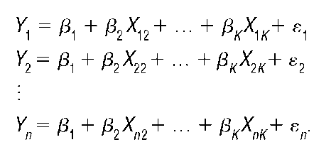
In the more general case where K> 2, it is useful to think of the model in (2) as a system of equations, such as:
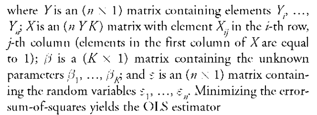
This can be written in matrix form as
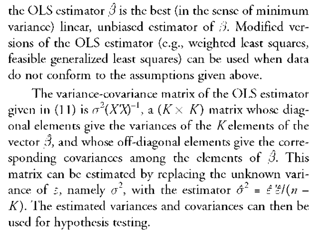
The Gauss-Markov theorem establishes that provided i. the relationship between Y and X is linear as described by (10); ii. the elements of X are fixed, nonstochastic, and there exists no exact linear relationship among the columns of X; and
DISCOVERY OF THE METHOD
Robin L. Plackett (1972) and Stephen M. Stigler (1981) describe the debate that exists over who discovered the OLS method. The first publication to describe the method was Adriene Marie Legendre’s Nouvelles methodes pour la determination des orbites des cometes in 1806, followed by publications by Robert Adrain (1808) and Carl Friedrich Gauss ([1809] 2004). However, Gauss made several claims that he developed the method as early as 1794 or 1795; Stigler discusses evidence that supports these claims in his article "Gauss and the Invention of Least Squares" (1981).
Both Legendre and Gauss considered bivariate models such as the one given in (8), and they used OLS to predict the position of comets in their orbits about the sun using data from astronomical observations. Legendre’s approach was purely mathematical in the sense that he viewed the problem as one of solving for two unknowns in an overdetermined system of n equations. Gauss ([1809] 2004) was the first to give a probabilistic interpretation to the least squares method. Gauss reasoned that for a sequence Y1, …, Y of n independent random variables whose density functions satisfy certain conditions, if the sample mean
is the most probable combination for all values of the random variables and each n > 1, then for some a2 > 0, the density function of the random variables is given by the normal, or Gaussian, density function
In the nineteenth century, this was known as the law of errors. This argument led Gauss to consider the regression equation as containing independent, normally distributed error terms.
The least squares method quickly gained widespread acceptance. At the beginning of the twentieth century, Karl Pearson remarked in his article in Biometrika (1902, p. 266) that "it is usually taken for granted that the right method for determining the constants is the method of least squares." Beginning in the 1870s, the method was used in biological, genetic applications by Pearson, Francis Galton, George Udny Yule, and others. In his article "Regression towards Mediocrity in Hereditary Stature" (1886), Galton used the term regression to describe the tendency of the progeny of exceptional parents to be, on average, less exceptional than their parents, but today the term regression analysis has a rather different meaning.
Pearson provided substantial empirical support for Galton’s notion of biological regression by looking at hereditary data on the color of horses and dogs and their offspring and the heights of fathers and their sons. Pearson worked in terms of correlation coefficients, implicitly assuming that the response and explanatory variables were jointly normally distributed. In a series of papers (1896, 1900, 1902, 1903a, 1903b), Pearson formalized and extended notions of correlation and regression from the bivariate model to multivariate models. Pearson began by considering, for the bivariate model, bivariate distributions for the explanatory and response variables. In the case of the bivariate normal distribution, the conditional expectation of Ycan be derived in terms of a linear expression involving X, suggesting the model in (8). Similarly, by assuming that the response variable and several explanatory variables have a multivariate normal joint distribution, one can derive the expectation of the response variable, conditional on the explanatory variables, as a linear equation in the explanatory variables, suggesting the multivariate regression model in (2).
Pearson’s approach, involving joint distributions for the response and explanatory variables, led him to argue in later papers that researchers should in some situations consider nonsymmetric joint distributions for response and explanatory variables, which could lead to nonlinear expressions for the conditional expectation of the response variable. These arguments had little influence; Pearson could not offer tangible examples because the joint normal distribution was the only joint distribution to have been characterized at that time. Today, however, there are several examples of bivariate joint distributions that lead to nonlinear regression curves, including the bivariate exponential and bivariate logistic distributions. Aris Spanos describes such examples in his book Probability Theory and Statistical Inference: Econometric Modeling with Observational Data. Ronald A. Fisher (1922, 1925) later formulated the regression problem closer to Gauss’s characterization by assuming that only the conditional distribution of the response variable is normal, without requiring that the joint distribution be normal.
CURRENT USES
Today, OLS and its variants are probably the most widely used statistical techniques. OLS is frequently used in the behavioral and social sciences as well as in biological and physical sciences. Even in situations where the relationship between dependent and explanatory variables is nonlinear, it is often possible to transform variables to arrive at a linear relationship. In other situations, assuming linearity may provide a reasonable approximation to nonlinear relationships over certain ranges of the data. The numerical difficulties faced by Gauss and Pearson in their day are now viewed as trivial given the increasing speed of modern computers. Computational problems are encountered, however, in problems with very large numbers of dimensions. Most of the problems that are encountered involve obtaining accurate solutions for the inverse matrix (XX)-1 using computers with finite precision; care must be taken to ensure that solutions are not contaminated by round-off error.


